Calibration of the LWIR16 camera prototype
$("#lwir_calibration").player(2);
Download links for: video and captions.
This research “Long-Range Thermal 3D Perception in Low Contrast Environments” is funded by NASA contract 80NSSC21C0175
Convert ip cam to web cam in Linux for Jitsi, Zoom, etc.
Basically, one need to direct the ip cam stream (mjpeg or rtsp) to a virtual v4l2 device which acts like a web cam and is automatically picked up by a web browser or a web cam application.
Quick setup Install and create a virtual webcam~$ sudo apt install v4l2loopback-dkms
~$ sudo modprobe v4l2loopback devices=1
The options below are for gstreamer/ffmpeg and rtsp/mjpeg streams:
gstreamer:
# rtsp stream
~$ sudo gst-launch-1.0 rtspsrc location=rtsp://192.168.0.9:554 ! rtpjpegdepay ! jpegdec ! videoconvert ! tee ! v4l2sink device=/dev/video0 sync=false
# mjpeg stream
~$ sudo gst-launch-1.0 souphttpsrc is-live=true location=http://192.168.0.9:2323/mimg ! jpegdec ! videoconvert ! tee ! v4l2sink device=/dev/video0
ffmpeg:
# rtsp stream
~$ sudo ffmpeg -i rtsp://192.168.0.9:554 -fflags nobuffer -pix_fmt yuv420p -f v4l2 /dev/video0
# mjpeg stream
~$ sudo ffmpeg -i http://192.168.0.9:2323/mimg -fflags nobuffer -pix_fmt yuv420p -r 30 -f v4l2 /dev/video0
Start a video conference application, select the webcam from the menu (/dev/video0).
Test link: meet.jit.si
- ffmpeg (2.8.15) or gstreamer (1.8.3)
- IP camera capable of streaming mjpeg or rtsp – in this case it’s Elphel NC393
- rtsp stream ports for Elphel NC393 cameras: 554, 556, 558, 560
- mjpeg stream ports for Elphel NC393 cameras: 2323, 2324, 2325, 2326
- stream resolution/fps: 1920×1080, 30fps
- ffmpeg for mjpeg stream – “-r 30” sets fps – the default ffmpeg setting is 25 fps
Print web cam settings:
v4l2-ctl -d 0 --all
Gstreamer play mjpeg:
gst-launch-1.0 souphttpsrc is-live=true location=http://192.168.0.9:2323/mimg ! jpegdec ! autovideosink
Gstreamer play rtsp:
gst-launch-1.0 -v playbin uri=rtsp://192.168.0.9:554 uridecodebin0::source::latency=0
Test stream for web cam:
sudo gst-launch-1.0 videotestsrc ! tee ! v4l2sink device=/dev/video0
- Gstreamer 1.8.3 didn’t work without tees in the pipeline.
- modprobe v4l2loopback can create multiple devices
TPNET with LWIR
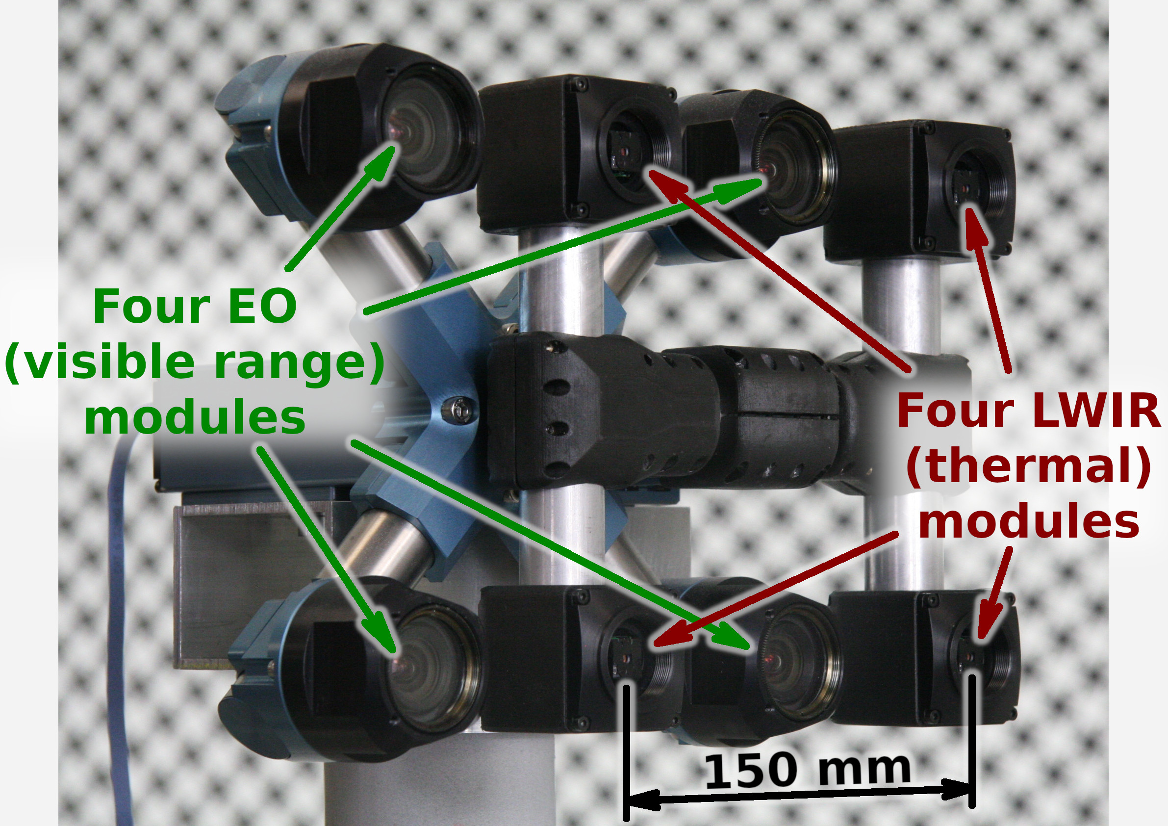
Figure 1. Talon (“instructor/student”) test camera.
SummaryThis post concludes the series of 3 publications dedicated to the progress of Elphel five-month project funded by a SBIR contract.
After developing and building the prototype camera shown in Figure 1, constructing the pattern for photogrammetric calibration of the thermal cameras (post1), updating the calibration software and calibrating the camera (post2) we recorded camera image sets and processed them offline to evaluate the result depth maps.
The four of the 5MPix visible range camera modules have over 14 times higher resolution than the Long Wavelength Infrared (LWIR) modules and we used the high resolution depth map as a ground truth for the LWIR modules.
Without machine learning (ML) we received average disparity error of 0.15 pix, trained Deep Neural Network (DNN) reduced the error to 0.077 pix (in both cases errors were calculated after removing 10% outliers, primarily caused by ambiguity on the borders between the foreground and background objects), Table 1 lists this data and provides links to the individual scene results.
For the 160×120 LWIR sensor resolution, 56° horizontal field of view (HFOV)and 150 baseline disparity of one pixel corresponds to 21.4 meters. That means that at 27.8 meters this prototype camera distance error is 10%, proportionally lower for closer ranges. Use of the higher resolution sensors will scale these results – 640×480 and longer baseline of 200 mm (instead of the current 150 mm) will yield 10% accuracy at 150 meters, 56°HFOV.
Table1: LWIR 3D disparity measurement accuracy enhanced by TPNET deep neural network (DNN). # Scene timestamp and comments [Expand all] Non-TPNET disparity error (pix) TPNET disparity error (pix) TPNET accuracy gain 1 1562390202_933097: Single person, trees. EO(m) LWIR(m) Err(%) 16.2 16.5 1.64 10.2 10.1 -1.13 17.7 18.4 3.93 51.2 46.5 -9.17 20.6 19.7 -4.47 Detailed results page (pdf) 0.136 0.060 2.26 2 1562390225_269784: Single person, trees. EO(m) LWIR(m) Err(%) 16.5 16.4 -0.04 26.0 27.5 5.98 9.2 9.8 7.41 6.3 6.2 -0.62 Detailed results page (pdf) 0.147 0.065 2.25 3 1562390225_839538: Single person. Horizontal motion blur. EO(m) LWIR(m) Err(%) 9.1 8.3 -8.65 5.5 5.7 2.54 35.8 37.6 4.88 14.9 16.1 7.95 Detailed results page (pdf) 0.196 0.105 1.86 4 1562390243_047919: No people, trees. EO(m) LWIR(m) Err(%) 7.5 7.2 -3.31 9.9 10.2 2.53 27.2 26.6 -2.41 108.7 95.2 -12.42 121.3 143.3 18.16 6.3 6.3 -0.68 9.8 10.1 3.52 Detailed results page (pdf) 0.136 0.060 2.26 5 1562390251_025390: Open space. Horizontal motion blur. EO(m) LWIR(m) Err(%) 8.1 7.9 -2.80 19.7 21.0 6.86 25.6 27.1 5.90 8.2 8.2 -0.06 47.6 48.9 2.70 107.3 96.9 -9.71 23.0 21.5 -6.40 Detailed results page (pdf) 0.152 0.074 2.06 6 1562390257_977146: Three persons, trees. EO(m) LWIR(m) Err(%) 10.0 9.6 -3.73 9.1 8.8 -3.11 6.9 7.0 1.38 11.4 11.3 -1.00 8.7 8.6 -1.07 Detailed results page (pdf) 0.146 0.074 1.96 7 1562390260_370347: Three persons, near and far trees, minivan. EO(m) LWIR(m) Err(%) 11.1 10.7 -3.34 10.4 10.4 0.12 8.7 8.8 1.14 11.3 11.4 0.56 8.5 8.6 1.69 11.3 11.3 -0.83 32.8 34.2 4.29 91.6 84.9 -7.23 49.8 47.9 -3.80 130.0 140.7 8.26 51.9 54.6 5.35 Detailed results page (pdf) 0.122 0.058 2.12 8 1562390260_940102: Three persons, trees. EO(m) LWIR(m) Err(%) 11.8 11.0 -6.45 10.7 10.3 -3.76 8.7 9.1 4.98 11.3 11.4 0.18 8.6 8.5 -1.87 11.0 11.2 2.27 31.4 35.3 12.25 27.9 29.6 6.31 Detailed results page (pdf) 0.135 0.064 2.12 9 1562390317_693673: Two persons, far trees. EO(m) LWIR(m) Err(%) 9.5 9.4 -0.65 11.0 11.3 2.28 66.8 76.6 14.66 95.0 79.1 -16.75 81.9 93.0 13.45 69.4 72.8 4.83 9.8 9.4 -3.67 Detailed results page (pdf) 0.157 0.078 2.02 10 1562390318_833313: Two persons, trees. EO(m) LWIR(m) Err(%) 8.3 8.3 -0.67 10.6 10.7 1.00 81.2 78.7 -3.17 63.6 48.4 -23.98 86.2 78.9 -8.46 54.0 53.4 -1.10 12.0 11.8 -1.61 76.9 80.0 3.94 23.3 28.4 21.99 Detailed results page (pdf) 0.136 0.065 2.10 11 1562390326_354823: Two persons, trees. EO(m) LWIR(m) Err(%) 6.5 6.2 -4.85 9.2 9.4 2.86 21.3 21.0 -1.36 6.9 7.1 2.15 19.7 19.1 -3.08 Detailed results page (pdf) 0.144 0.090 1.60 12 1562390331_483132: Two persons, trees. EO(m) LWIR(m) Err(%) 5.4 5.1 -5.19 8.1 8.1 0.03 6.9 6.8 -1.09 5.9 6.0 1.29 16.4 15.9 -2.72 Detailed results page (pdf) 0.209 0.100 2.08 13 1562390333_192523: Single person, sun-heated highway fill. EO(m) LWIR(m) Err(%) 4.3 4.2 -2.32 10.6 10.5 -0.75 6.7 6.8 0.51 20.2 19.1 -5.67 14.7 14.3 -2.81 18.1 19.0 4.60 Detailed results page (pdf) 0.153 0.067 2.30 14 1562390402_254007: Car on a highway, background trees. EO(m) LWIR(m) Err(%) 11.9 11.9 0.30 31.1 29.6 -5.05 27.6 28.1 1.66 30.6 35.1 14.51 Detailed results page (pdf) 0.140 0.077 1.83 15 1562390407_382326: Car on a highway, background trees. EO(m) LWIR(m) Err(%) 12.0 12.3 2.53 30.7 29.3 -4.47 27.3 25.6 -6.30 29.9 30.2 1.14 27.4 34.5 25.73 Detailed results page (pdf) 0.130 0.065 2.01 16 1562390409_661607: Single person, a car on a highway. EO(m) LWIR(m) Err(%) 9.5 9.5 -0.35 28.3 32.1 13.44 124.5 88.7 -28.74 29.4 31.4 6.72 14.4 14.9 3.24 Detailed results page (pdf) 0.113 0.063 1.79 17 1562390435_873048: Single person, two parked cars. EO(m) LWIR(m) Err(%) 7.8 7.9 1.18 22.2 22.4 0.85 56.9 65.3 14.91 121.4 113.0 -6.96 Detailed results page (pdf) 0.153 0.057 2.68 18 1562390456_842237: Close trees. EO(m) LWIR(m) Err(%) 9.6 9.5 -1.69 6.7 6.5 -2.49 114.6 96.0 -16.25 7.4 7.4 0.26 8.1 8.0 -1.49 Detailed results page (pdf) 0.211 0.102 2.08 19 1562390460_261151: Trees closer than the near clipping plane. EO(m) LWIR(m) Err(%) 5.4 5.4 0.76 3.9 3.8 -0.53 4.2 4.3 3.01 4.9 5.0 3.48 100.1 82.5 -17.59 Detailed results page (pdf) 0.201 0.140 1.44 Average 0.154 0.077 2.04
Notes: click on the scene title to show details. Click on the image to start/stop GIF animation.
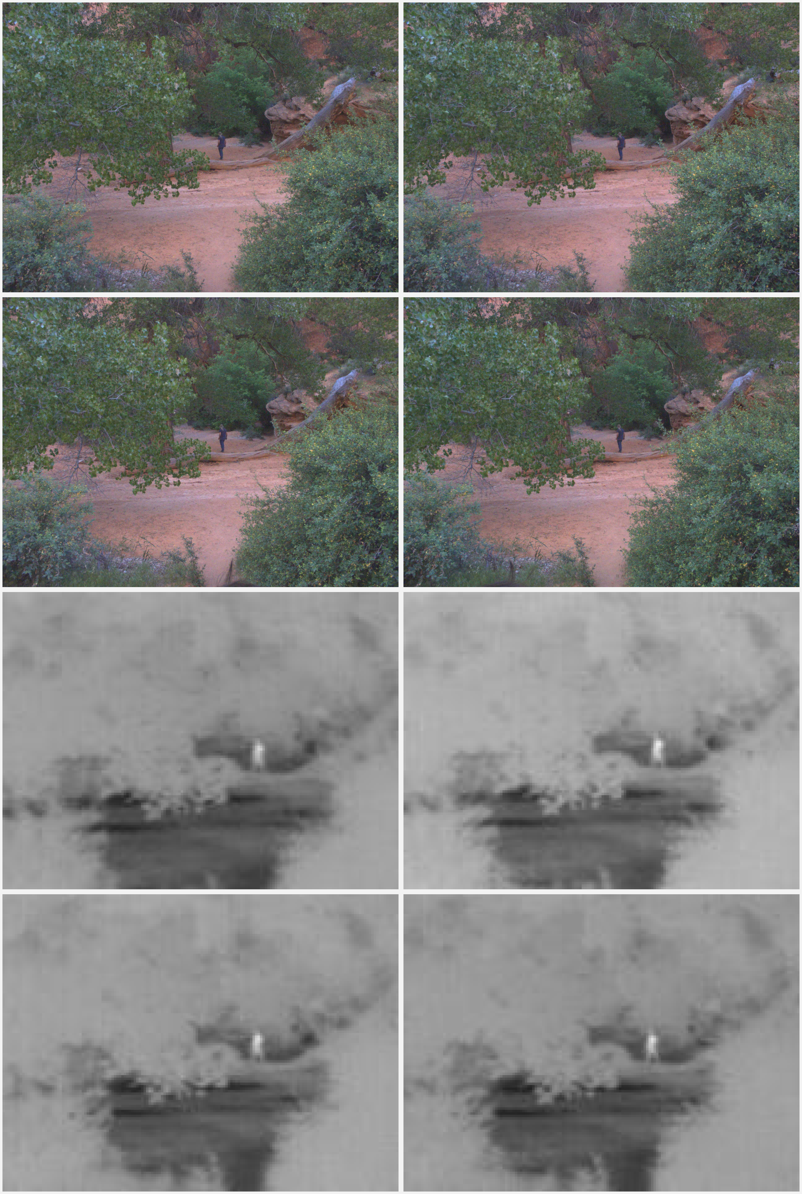
Detailed resultsFigure 2 illustrates results at the output and at the intermediate processing steps. Similar data is availble for each of the 19 evaluated scenes listed in the Table 1 (Figure 2 corresponds to scene 7, highlighted in the table).
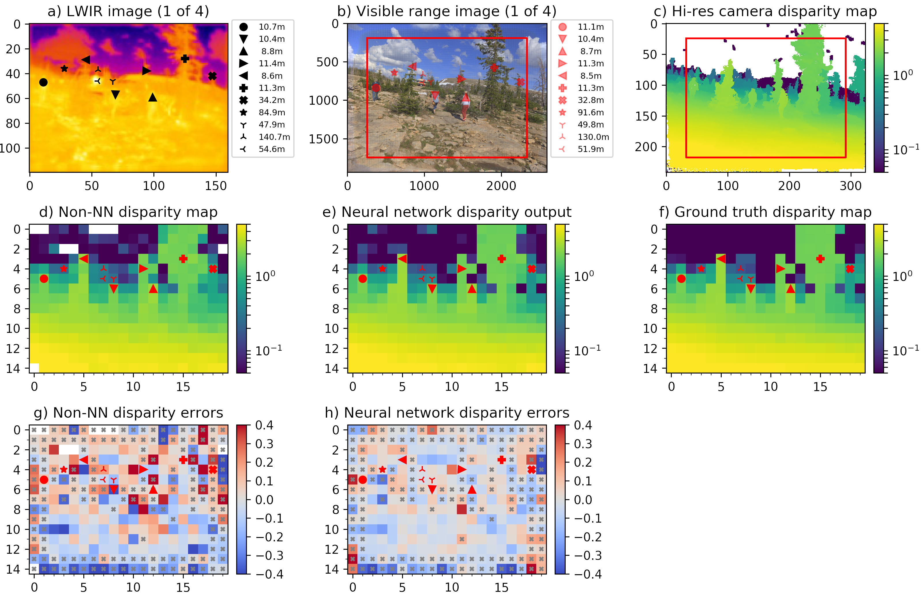
Figure 2. LWIR depth map generation and comparison to the ground truth data.
Processing steps to generate and evaluate LWIR depth mapsFour visible range 5 Mpix (2592×1936) images (Figure 2b) are corrected from the optical aberrations and are used to generate disparity map c) that has 1/8 resolution (324×242 where each pixel corresponds to an overlapping 16×16 tile in the source images) with the Tile Processor. Red frames in b) and c) indicate field of view of the LWIR camera modules. Each of the high resolution disparity tiles in c) is mapped to the corresponding tiles of the 20×15 LWIR disparity map f). This data is used as ground truth for both neural network training and subsequent testing and inference (20% of the captured 1100 image sets are reserved for testing, 80% are used for training).
One of the 4 simultaneously acquired LWIR images is shown in Figure 2a. Table 1 contains animated GIFs for each set of 4 scene images, animation (click image to start) consequently shows all 4 views of the quad camera setup. These 4 LWIR images are partially rectified and then subject to 2D correlation between each of the 6 image pairs, resulting in the disparity map d) similarly to how it is done for the visible range (aka electro-optical or EO) ones. Sub-plot g) shows the difference between LWIR disparity map calculated without machine learning d) and the ground truth data f). Subplot e) contains disparity map enhanced by the ML that uses raw 2D-correlation data (Figures 3, 4) as its input features. And the last subplot h) shows difference between e) and f) as the resudual errors after full TPNET processing. Manually placed markers listed in a) and b) correspond to the scene features, black markers in a) show linear distances calculated from the output e), while red markers legend in b) lists the corresponding ground truth distances. Table 1 contain the same data and additionally shows relative errors of the LWIR measurements.
Gray “×”-es in g) and h) indicate tiles where data may be less reliable. These tiles include 2-tile margins on each side of the map, caused by the fact that convolution part of the neural network analyses 5×5 tile clusters. Bottom edge tiles use pixels that are not available in top pair of the four images because of the large parallax for the near objects, so bottom tiles use only a single binocular pair instead of the 6 available for the inner tiles.
Another case of the potential mismatch between the disparity output and the ground truth data is when different range objects in high-resolition map c) correspond to the same tile in LWIR maps d) and e). The network is trained to avoid averaging of the far and near objects in the same tile, but it still can wrongly identify which of the planes (foreground or background) was selected for the ground truth map. For this reason all LWIR tiles that have both foreground and background match in c) are also marked.
Most of the tiles that have both foreground and background objects are assigned corectly so we do not remove the marked tiles from the average error calculation. Instead we handle gross outliers by discarding a fixed fraction of all tiles (we used 10%) that have the largest disparity errors and average errors among the remaining 90% of tiles.
Depth maps X/Y resolutionDisparity maps generated from the low resolution 160×120 LWIR sensors of the prototype camera have even lower resolution of just 20×15 tiles. There are other algorithms that generate depth maps with the same pixel resolution as the original images, but they have lower ranging accuracy. Instead we plan to fuse high-reolution (pixel-accurate) rectified source images and low X/Y (but high Z) resolution depth maps with another DNN. That was not a part of this project, but it is doable — similar approach is already used for fusion of the high-resolution regular images with the low pixel resolution time-of-flight (ToF) cameras or LIDARs. Deep subpixel resolution needed for the ranging accuracy requires many participating pixels for each object no be measured, so the fusion will not significantly increase the number of different objects in each tile, but it can restore the pixel accuracy of the object contours.
Comments on the individual scenesAmong the evaluated scenes there are two with strong horizontal motion blur caused by the operator turning around the vertical axis – scenes 3 and 5. Such blur can not be completely eliminated by the nature of the microbolometer sensors, so the 3D perception has to be able to mitigate it. If it was just a traditional binocular system, horizontal blur would drown useful data in the noise and make it impossible to achieve a deep subpixl resolution. Quad non-colinear stereo layout is able to mitigate this problem and the acuracy drop is less prominent.
The last two scenes (18 and especially 19) demonstrate high disparity errors (0.1 and 0.14 pixels respectively). These large errors correspond to high absolute disparity value (over 8 pix) and low distances (under 3 meters) where disparity variations within the same tile are high and so the disparity of a tile is ambiguous. On the other hand, relative disparity error for even 0.4 pixels is only 5% or just 15 cm at 3 m range. Scene 19 has details in the right side that are closer than the near clipping plane preset for of the ground truth camera.
TPNET – Tile Processor with the deep neural network Image rectification and 2D correlationEarlier post “Neural network doubled effective baseline of the stereo camera” (and also arXiv:1811.08032 preprint) explains the process of aberration correction, partial rectification of the source images and calcualtion of the 2D phase correlation using Complex Lapped Transform (CLT) for the 16×16 overlapping tiles (stride 8) of the quad camera high resolution visible range images. We used the same algorithms in the current project too. Depth perception with TPNET is a 2-step process (actually iterative as these steps may need be repeated) similar to the human stereo vision – first the eyes are converged at the objects at certain distance producing zero disparity between the two images there, then data from the pair of images is processed (locally in retinas and then in the visual cortex) to extract residual mismatch and convert it to depth. There are no moving parts in TPNET-based system, instead the Tile Processor implements target disparity (“eye convergence”) by image tile shifts in the frequency domain with CLT, so it is as if each of the image tiles had a set of 4 small “eyes” that simultaneously can converge at different distances.
Figure 3. Set of four images of the scene 7. (click to start/stop)
Figure 3 shows partially rectified set of 4 LWIR images of the scene 7. “Partially” means that they are not rectified to the complete rectilinear (pinhole) projection, but are rather subject to subtle shifts to a common to all four of them radial distortion model. CLT is similar to 2D Fourier transform and is also invariant to shifts, but not to stretches and rotations. We use subpixel-accurate tile shifts in the frequency domain, benefitting from the fact that individual lenses while different have similar focal length and distortion parameters. Complete distortion correction would require image resampling increasing computation load and memory footprint or reducing subpixel resolution.
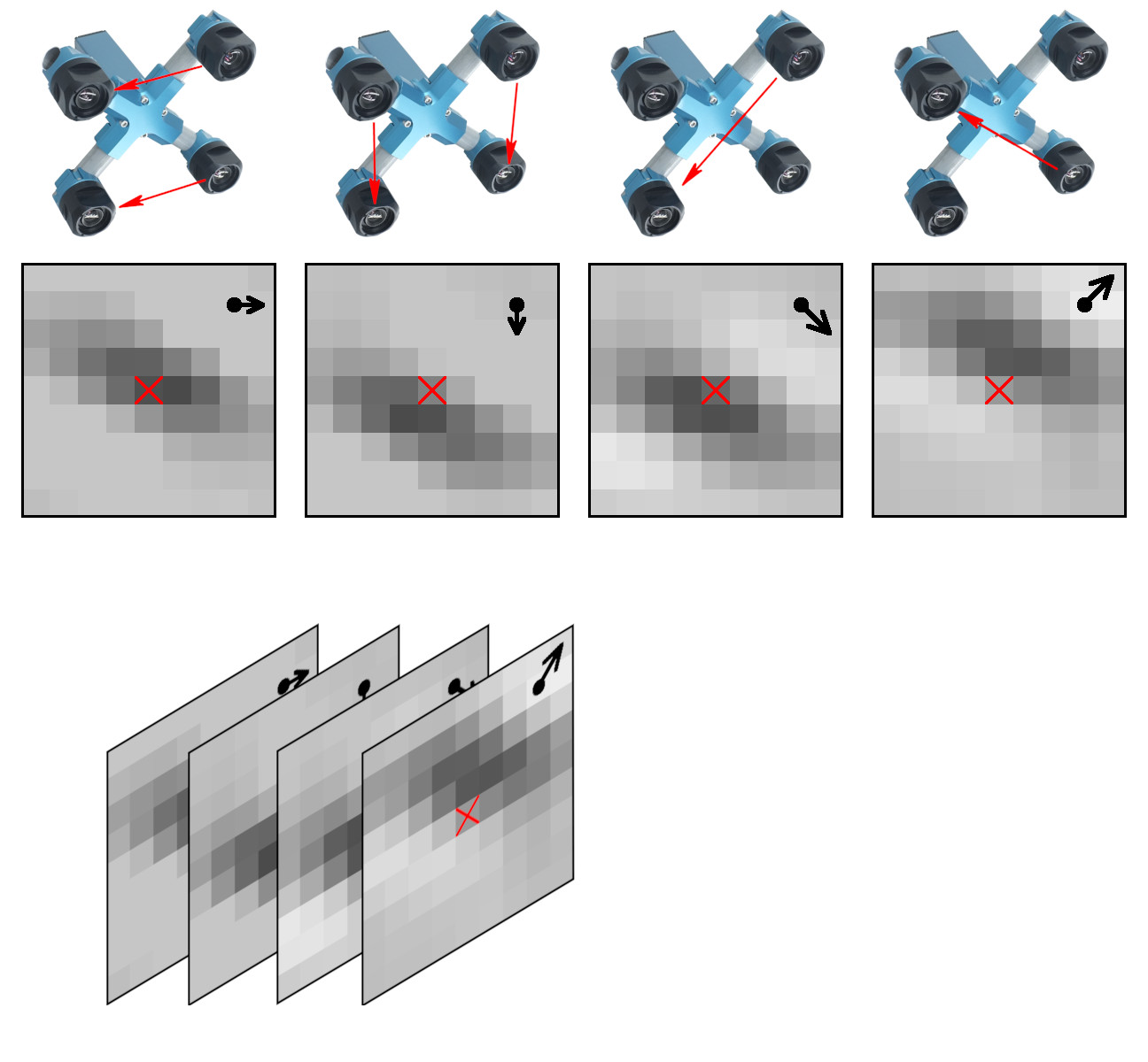
Next two figures contain 2D phase correlation data that is fed to the DNN part of TPNET. Figure 4 is calculated with each tile target disparity of zero (converged at infinity). The four frames of the GIF animation correspond to 4 stereo pairs directions – horizontal, vertical and 2 diagonals, as indicated in the top left image corner.
Figure 4. 2D phase correlations with all tiles target disparity set to 0. (click to start/stop)
Figure 5. 2D phase correlations, target disparity set by the polynomial approximaton. (click to start/stop)
Similarly to the source images (Figure 3) all the correlation tiles for infinity objects (as clouds in the sky) do not move when animation is running, while the near objects do – the residual disparity (diffenece beween the full disparity and the “target disparity”) value corresponds to the offest of the spot center from the grid center in the dirrection of the red arrows. The correlation result is most accurate when residual disparity is near zero, the farther the spot center is from zero, the less source pixels participate in matching and so the correlation S/N ratio and resolution drop.
Figure 5 is similar, but this time each tile target disparity is set by the iterative process of finding residual correlation argmax by the polynomial approximation and re-calculating new 2D correlation. This time most of the tiles do not move, except those that are on the foreground/backgroud boreders.
Neural network layout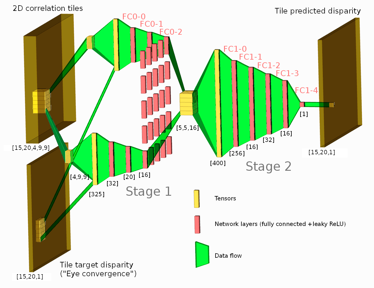
Figure 6. Network diagram
The 2D phase correlation tiles shown above and the per-tile target disparity value make the input features that are fed to the neural network during training and later inference. We tried the same network architecture and cost finctions we developed for the high resolution cameras (blog post, arXiv:1811.08032 preprint) and it behaved really well, allowing us to finish this project in time.
The network consists of two stages, where the first one gets input features from a single tile 2D phase correlation as [4,9,9] tensor (first dimension, 4 is the number of correlation pairs, two others (9×9) specify the center window of the full 15×15 2D correlation – 4 pixels in each direction around the center). Stage 1 output for each tile is a 16-element vector fed to the Stage 2 inputs.
Stage 2 subnet for each tile gets input features from the corresponding stage 1 output and its 24 neighbors in a form of a [5,5,16] tensor. The output of the stage 2 is a single scalar for each tile or [15,20,1] tensor for the whole disparity map, shown in Figure 2e. Such two-stage layout is selected to allow the network to use neighbor tiles when generating its disparity output (such as to continue edges, to fill low-textured areas, and to improve foreground/background separation), but simultaneously limit dimensions of the fully connected layers.
Training and the cost functionInstead of the full images the training sets consist of the 5×5 tile fragments harvested from the 880 image sets. Randomly constructed batches use 2D histogram normalization of the image tiles, so each batch includes similar repesenation of near and far, high contrast and low contrast tiles. Cost function design followed the same approach as described in the earlier post, we clipped the L2 cost of the difference with ground truth (essentially giving up on gross outliers caused by incorrect foreground/background tiles assignment) and included additional terms.
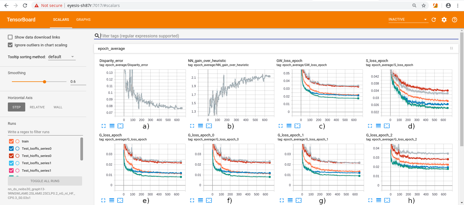
Figure 7. Screenshot of the Tensorboard after TPNET training. a) test image average disparity error; b) network accuracy gain over heuristic (non-NN); c) total cost function; d) cost of “cutting corners” between the foreground and background; e) cost of mixture of L2 for 5×5, 3×3 and single tile Stage2; f) cost for 5×5 only (used for inference); g) cost for 3×3 only; h) cost for single tile only.
Additional cost function terms included regularization to reduce overfitting, and the one to avoid averaging of the distances to the foreground and background objects for the same tile, forcing the network to select either fore- or background, but not their mixture.
Regularization included “shortcuts” requiring that if just a single (center) tile input from Stage 1 is fed to stage 2, it should provide less accurate but still reasonably good disparity output (Figure 7h), same for the 3×3 sub-window (Figure 7g). Only full 5×5 Stage 2 output (Figure 7f) is used for test image evaluation and inference, but training uses a weighted mixture of all three (Figure 7e).
Cost function term to reduce averaging of foreground and background disparities in the border tiles (Figure 7d) is made in the following way: for each tile the average of the ground truth disparities of its 8 neighbors is calculated, and additional cost is imposed if the network output falls between the ground truth and this average. Figure 7c shows the total cost function that combines all individual terms.
Conclusion- Experiments with the prototype LWIR 3D camera provided disparity accuracy consistent with our earlier results obtained with the high resolution visible range cameras.
- The new photogrammetric calibration pattern design is adequate for the LWIR imaging and can be used for factory calibration of the LWIR cameras and camera cores.
- Machine learning with TPNET provided 2× ranging accuracy improvement over the one obtained with the same data and traditional only (w/o machine learning) processing.
- Combined results proved the feasibility of completely passive LWIR 3D perception even with relatively low resolution thermal sensors.
Photogrammetric Calibration of the Quad Thermal Camera
Figure 1. Calibration of the quad visible range + quad LWIR camera.
We’ve got the first results of the photogrammetric calibration of the composite (visible+LWIR) Talon camera described int the previous post and tested the new pattern. In the first experiments with the new software code we’ve got average reprojection error for LWIR of 0.067 pix, while the visible quad camera subsystem was calibrated down to 0.036 pix. In the process of calibration we acquired 3 sequences of 8-frame (4 visible + 4 LWIR) image sets, 60 sets from each of the 3 camera positions: 7.4m from the target on the target center line, and 2 side views from 4.5m from the target and 2.2 m right and left from the center line. From each position camera axis was scanned in the range of ±40° horizontally and ±25° vertically.
In the first stage of calibration the acquired images (Figure 2 shows both LWIR and visible range images) were processed to extract the detected pattern grid node. Each node’s pixel coordinates (x,y), a pair of the pattern UV indexes and the contrast are stored in the form of multi-layer TIFF files – processed images from Figure 2 are shown on animated GIFs, Figure 3 is for LWIR and Figure 4 – for the visible range images. Each of the images has a link to a respective TIFF file that has metadata visible with ImageJ program.
Figure 2. LWIR and visible range images of the pattern.
The software for the calibration had to be modified, as it did not have provisions for handling different resolution sensors in the same system. Additionally it was designed for the smaller pattern cell size so each image had larger number of detected nodes. We also had to use other method of absolute pattern matching (finding out which of the multiple almost identical measure nodes corresponds to the particular (e.g. center) node of the physical pattern. Earlier, with the fine pitch patterns, we used software-controlled laser pointers, with the current approach we used the fact that the visible subsystem was already calibrated – that provided sufficient data for absolute matching. Only one image for each camera position had manually marked center pattern cell – that mark simplified the processing.
Before LWIR data was used the visible rage images were processed with Levenberg-Marquardt algorithm (LMA) and the system knew precise position and orientation of the camera during capturing of each image set. After preliminary adjustment with idealized (uniform and flat) pattern grid it was possible to simultaneously refine each physical pattern node location in 3d, similarly as we did earlier (Figures 4 and 5 in this post). Using large cell pattern, the visible cameras bundle adjustment resulted in 0.11 pixels when using just radial distortion model. This was improved to 0.036 pix when using non-radial correction to compensate other irregularities of the lenses.
When LWIR data was added and each image set had known extrinsic parameters, the absolute grid matching was performed in the following way. Starting with the image with the smallest distance from the target (so the wrong matching of the grid cell would cause attitude error larger than initial precision of the system assembly) the attitude angles of each of the 4 LWIR subcameras was found. Then for each additional image LMA was run with all but 2 parameters known and fixed – camera base position X and Y coordinates (in the plane parallel to the target). As the position was already known from the visible range subsystem, the X and Y difference was matched to the physical pattern dimensions to determine how many cells (if any) the assumed grid match is offset. That gave absolute grid match for all of the LWIR images, and bundle adjustment of the LWIR modules intrinsic (focal length, offset from the center pixel, radial distortion coefficient) as well as the modules location in the camera coordinate system and their attitudes was possible. It resulted in 0.097 pixels reprojection error with just the radial distortion model. We did not expect much from the non-radial correction as the sensor resolution is low, but it still gave some improvement – the residual error dropped down to 0.067 pix. It is likely this value can be improved more with better tweaking of the processing parameters – the current result was achieved in the first run.
Figure 3. Processed pattern grid from LWIR data (click image to download ImageJ Tiff stack).
Figure 4. Processed pattern grid from visible range camera data (click image to download ImageJ Tiff stack).
These calibration results are not that exciting compared to what we will get with the LWIR 3D model reconstruction, but it gives us confidence that we are on the right track, and our goal is possible. Having a much higher resolution sub-system conveniently provides ground truth data for training of the neural network – something that was much more difficult to achieve with the high resolution visible range only systems.
3D Perception with Thermal Cameras
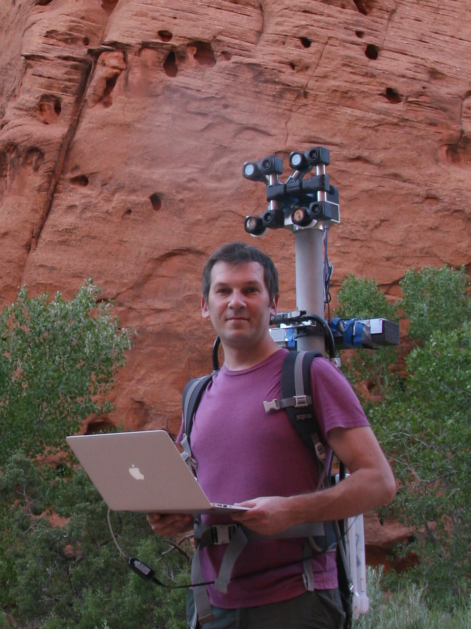
Figure 1. Oleg carrying combined LWIR and visible range camera.
While working on extremely long range 3D visible range cameras we realized that the passive nature of such 3D reconstruction that does not involve flashing lasers or LEDs like LIDARs and Time-of-Flight (ToF) cameras can be especially useful for thermal (a.k.a LWIR – long wave infrared) vision applications. SBIR contract granted at the AF Pitch Day provided initial funding for our research in this area and made it possible.
We are now in the middle of the project and there is a lot of the development ahead, but we have already tested all the hardware and modified our earlier code to capture and detect calibration pattern in the acquired images.
Printed Calibration Patterns for LWIR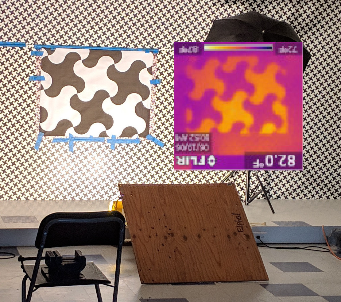
Figure 2. Initial LWIR pattern detection test with a small (100×100 pix) FLIR handheld camera.
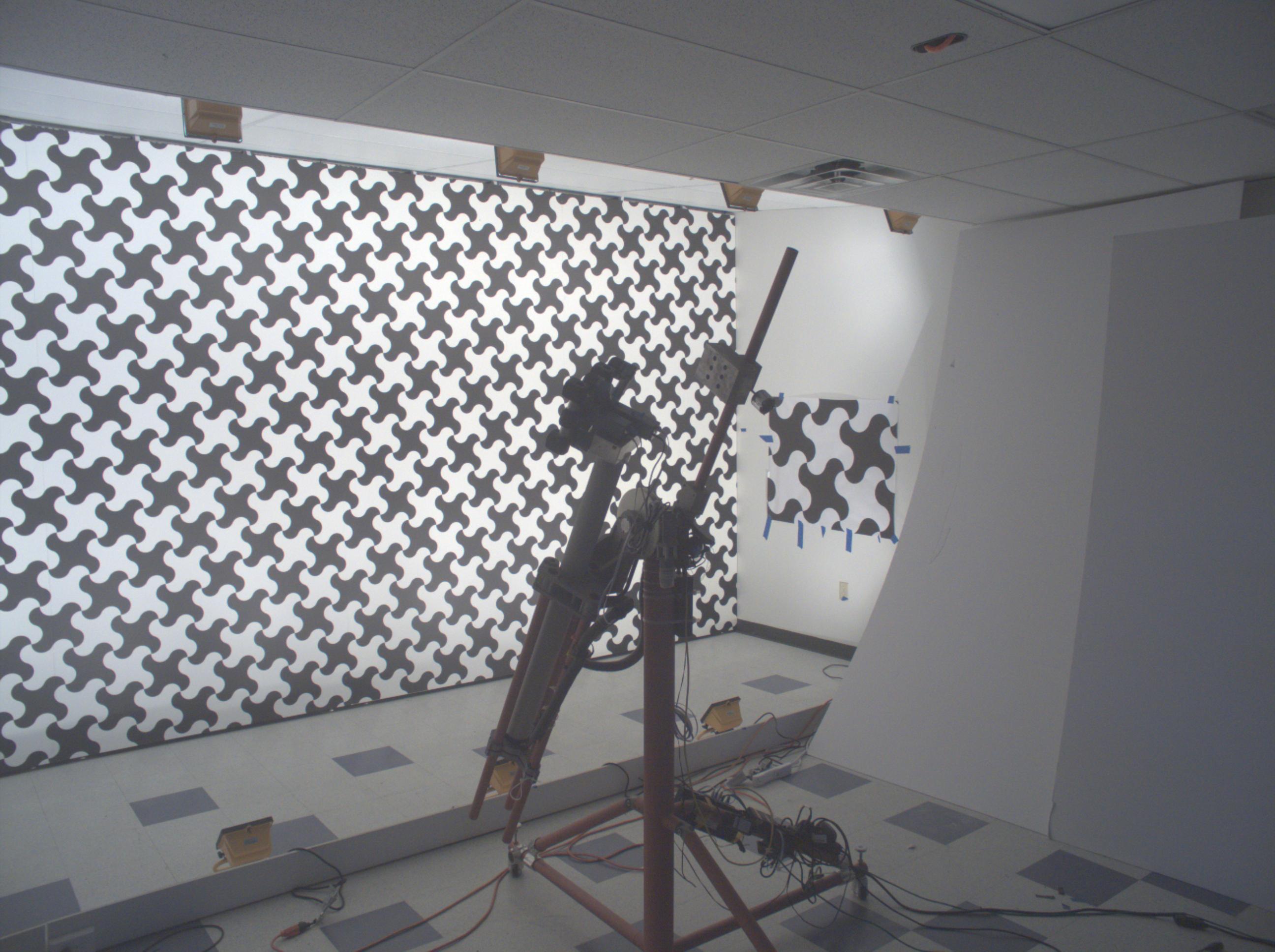
For the LWIR imaging we planned to use approach similar to what we have developed for the visible range cameras, and the first step is the precise photogrammetric camera calibration. Before engaging in the project we made sure that we can capture images of the pattern in LWIR wavelength range, the same pattern image should also be registered by the visible range camera to be used as the ground truth data. For the regular cameras there are many ways and materials to create high quality test patterns, our current setup uses 7.0 meters by 3.0 meters pattern printed on five sheets of self-adhesive film attached to the wall. This pattern illuminated by the regular bright fluorescent lamps did not register any image by a LWIR camera (we borrowed a small, handheld FLIR camera, used for HVAC applications).
In the next (successful) test we used a larger scale pattern printed on paper that was not bonded to the wall. The pattern was illuminated by a pair of 500W halogen lamps (see Figure 2). The lamp radiation — both visible and infrared (mostly infrared) was heating the image and so the black painted areas on paper became hotter than the white ones as shown in the FLIR camera image (it is upside down as the camera was held in a vise in that position). The measured temperature difference between white and black areas, illuminated from the distance of 1.5–2 meters was in the range of 2–4°K.
Figure 3. LWIR calibration pattern design.
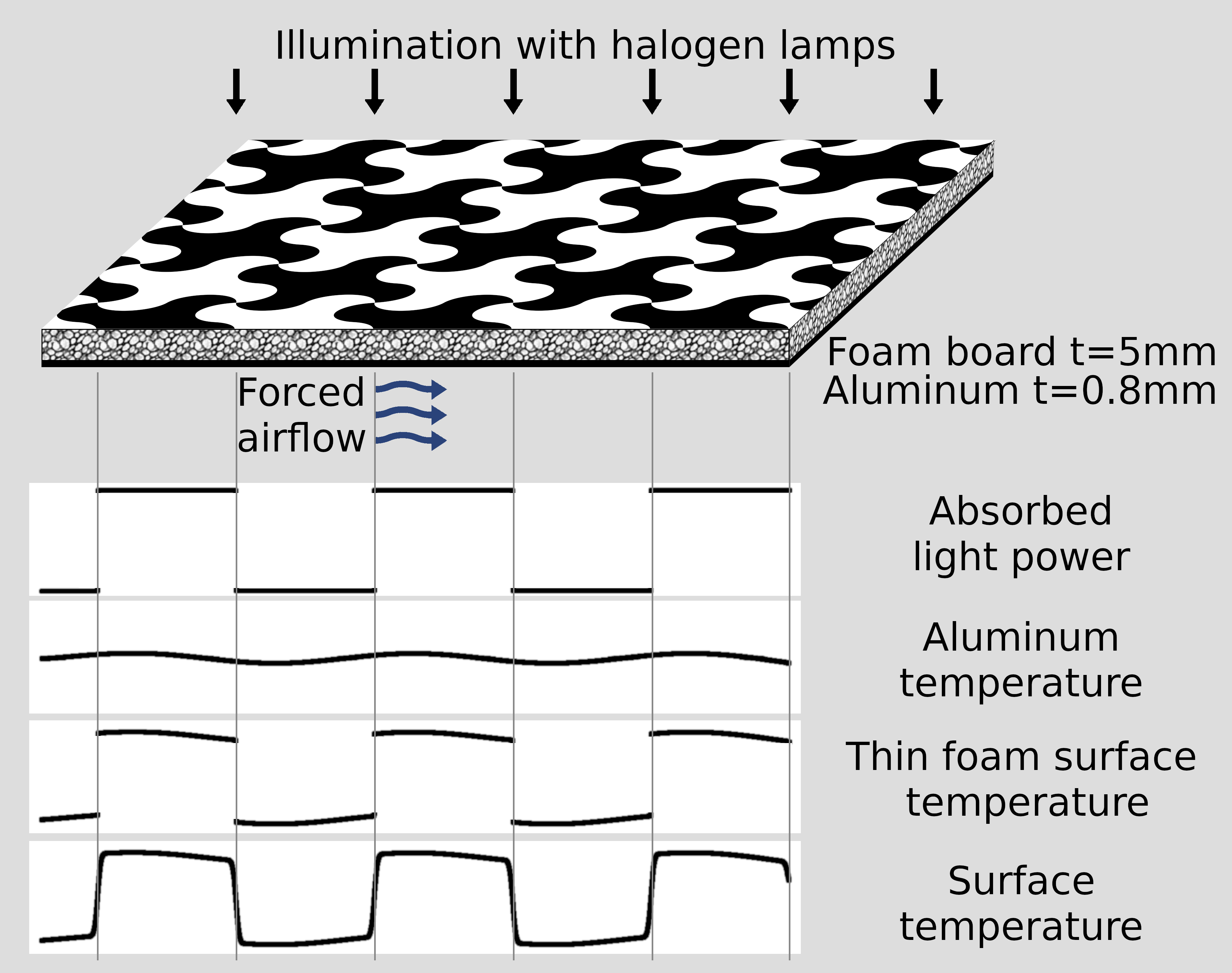
This quick test proved that with reasonable amount of high power halogen lamps we can achieve sufficient temperature contrast for the photogrammetric calibration. It still has some limitations — while the amount of heat absorbed by the pattern paint can be calculated from the data registered by the visible range cameras, the pattern surface temperature also depends on less controlled effects – air convection and heat transfer to the wall where the paper touches it. These factors reduce accuracy of the calibration, to mitigate their influence we designed a pattern where the ground truth relative surface temperature can be calculated from the measured visible range images and a few parameters that describe thermal properties of the materials.
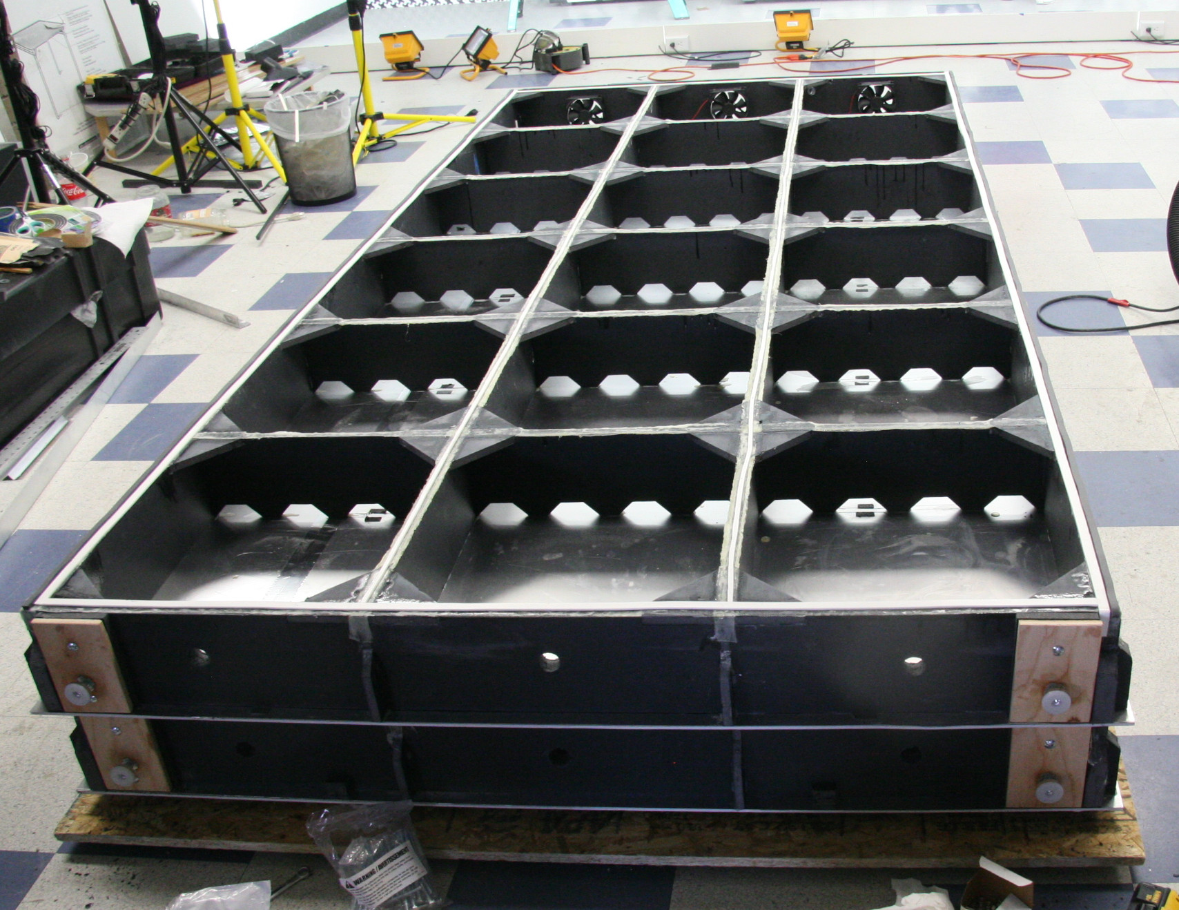
Calibration Pattern DesignWe used 5mm thick presentation type foam boards that consist of the polystyrene foam layer between two paper surface sheets. As we found out later, it is important to use both black and white paints during the printing process – unpainted paper surface that looks matte in visible light behaves like a mirror for the LWIR radiation and reflects the lamps used for illumination. You may find such reflection in Figure 5 – the leftmost panel that was built first does not have white paint. A thin (t=0.8 mm) aluminum sheets are glued to the back surfaces of the foam boards, and the forced airflow equalizes their temperatures. Figure 4 reveals the back side of the pattern module – thicker (1/2″ and 1″) machined foam boards make ribs that provide structural integrity of the pattern modules. These ribs are attached to the aluminum side of the pattern sheets with epoxy resin, their other side is reinforced with the fiberglass tape. Soft foam along the perimeter of the modules allows another use of the fans that provide the forced airflow – the developed vacuum is used to firmly press the modules to the smooth (covered with the visible range pattern film) wall. Timelapse video below illustrates the process of building and installation of the LWIR calibration pattern.
Figure 4. A stack of two face-down LWIR pattern modules.
Figure 3 illustrates temperature calculation for the uniformly illuminated pattern, this method will be used to derive ground truth thermal data from the registered visible range images. For a straight line on a surface of the pattern the absorbed light power produces a step function. The temperature of the underlying aluminum is a blurred version of that function, with the sigma depending on the thicknesses and thermal conductivity ratios of the foam and aluminum. With the used parameters amplitude of the aluminum temperature variations is below 1%. For the very thin foam the surface temperature would be just a sum of the aluminum temperature and a step function, the actual surface temperature distribution is blurred by the amount proportional to the foam thickness as the heat flow under the black/white pattern borders is not exactly orthogonal to the surface.
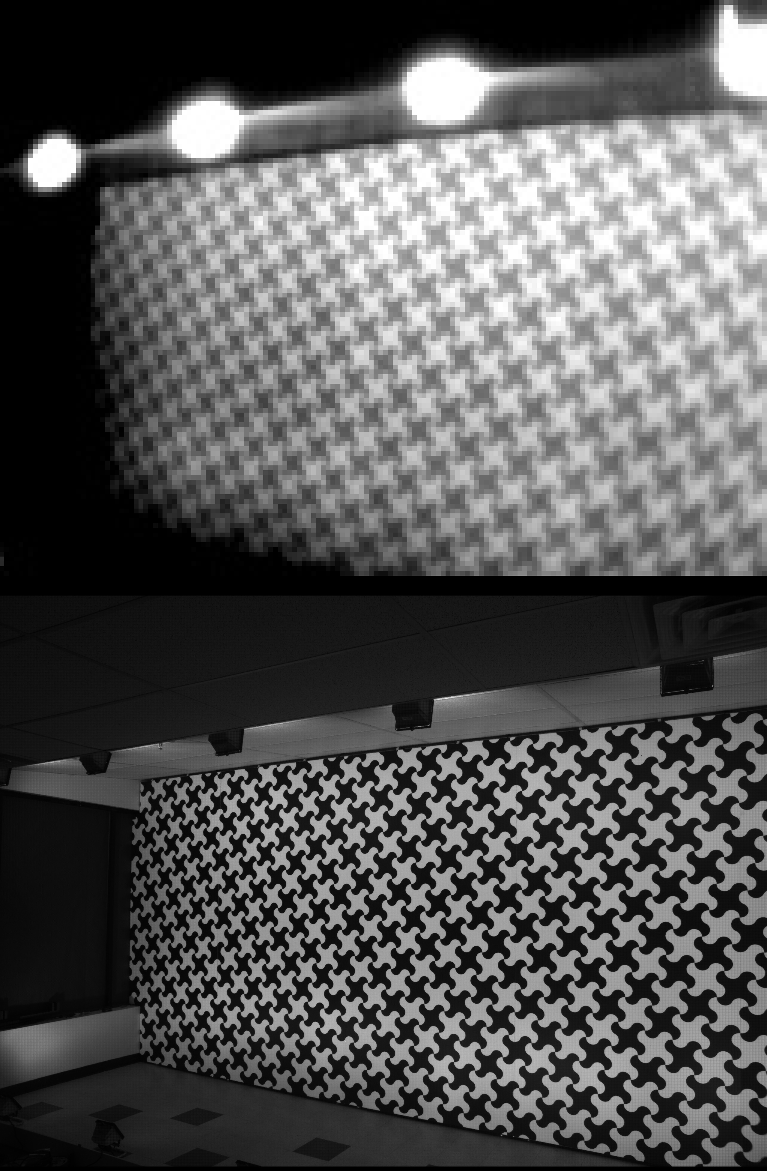
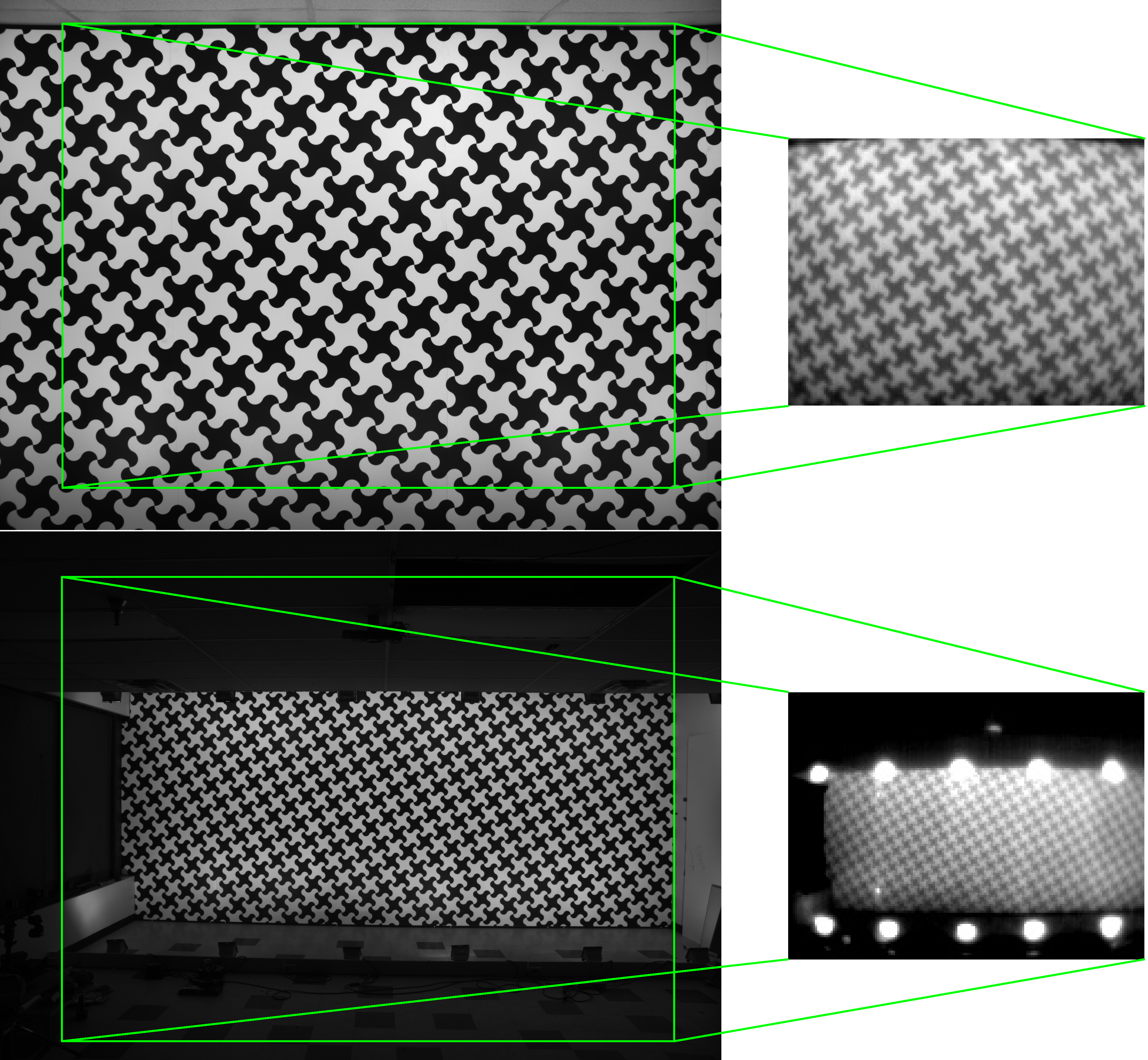
Calibration pattern period is 357mm, approximately four times larger than that of the pattern we use for the visible range cameras calibration. This size is selected to work with the low resolution prototype system (160×120 pix in each of the four channels) and still is suitable for the higher resolution LWIR imagers of up to 1280×960. Figure 5 shows the view of the pattern by the visible range (left) and LWIR (right) cameras from the distance of 3 meters (top) and 7 meters (bottom) from the target. The field of view of the already calibrated visible range cameras is slightly larger that that of the LWIR, so ground truth data is available over all LWIR sensors area.
Figure 5. LWIR calibration pattern captured by visible range (2592×1936) and LWIR (160×120) cameras from the distance of 3 meters (above) and 7 meters (below).
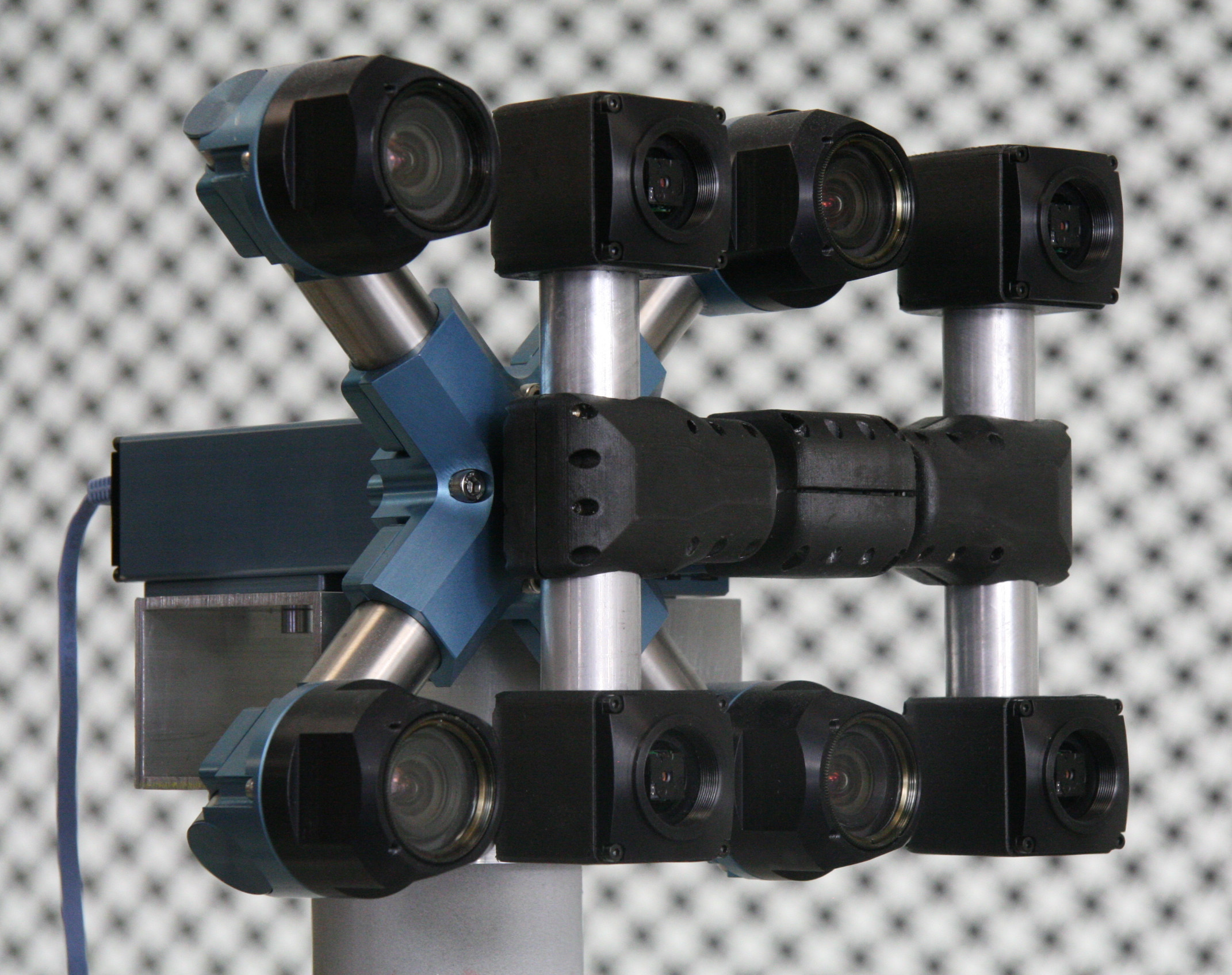
Visible + LWIR combo cameraThe main goal of our current project is to determine to what extent methods that we currently use for visible range camera photogrammetric calibration, distortion and aberration correction, deep subpixel disparity calculation and neural network training are applicable to the LWIR systems. Generally LWIR sensors have lower resolution than the regular visible and near infrared (VNIR) ones, are expensive and subject to export control, so with the limited time and resources available we selected small (160×120) FLIR Lepton-3.5 sensor modules available at Digi-Key. These modules have integrated germanium lenses and mechanical shutters that are essential for the photometric calibration. The sensors have limited frame rate (9 FPS) that puts them outside of the scope of export regulations. We plan use higher resolution sensors after evaluating the prototype system and achieving the goal of 0.1 pix (or better) disparity resolution.
The overall prototype camera design (Figure 6) is rather straightforward: we used already calibrated X-shaped quad camera and added another one with four LWIR sensors. FLIR Leton-3.5 modules do not support externally triggered operation, so I hoped that if all 4 sensors are fed with the same clock, and the reset signal is de-asserted simultaneously, then all channels will stay in sync and output frames simultaneously. Later this assumption turned out to be true, the difference between the channels after startup was in the range of ±10μs and it did not change over time. These small offset values are likely related to the analog PLL lock, they do not require any additional correction as they are more than a thousand times shorter than the effective pixel integration time. The visible range quad camera is triggered by the LWIR one. We measured internal LWIR module latency by capturing image of the rotating object and used this data to program the cameras triggering parameters to achieve simultaneous image capturing by all 8 of the visible range and thermal sensors.
Figure 6. Prototype combo camera: 4×VNIR+4×LWIR
Lepton-3.5 sensor module is small enough so we were able to fit it together with the power conditioning circuitry and the configuration EEPROM on the same dimension PCB as our regular sensor front ends (SFE) of 28mm×15mm and then mount in the standard SFE body. The board electrical and mechanical design is documented in Elphel Wiki.
Lepton module is controlled over the I2C bus that was already supported in Elphel NC393 series cameras, the video output is provided over SPI-based VoSPI interface, so some FPGA development along with the related drivers and applications code was required. Due to the digitized microbolometers output instead of that of a photodiodes in regular CMOS sensors, the rationale behind the use of the gamma compression that allows virtually lossless 8-bit representation of 12-bit pixel ADC output does not hold. That in turn required full 16-bit output rather than the JP4 image format that we were using for over a decade. We implemented Tiff format (both 8 and 16 bits per pixel) that is now available for all other supported image sensors, not only for the LWIR ones.
Photogrammetric calibration softwareWe are now working on adapting our existing code base to work with the LWIR low resolution sensors, and the photogrammetric calibration is the first step before we can perform 3D scene reconstruction and train a DNN to get higher disparity measurement accuracy. Our existing calibration workflow consists of the following steps:
- Capturing of a few hundred image sets of the calibration pattern from a 3 different camera locations, using switchable laser pointers for absolute matching of the periodic pattern cells in the camera images.
- Extracting pattern grid key points positions in the individual images with deep subpixel accuracy (0.03-0.05 pix) combining both pixel domain and frequency domain image processing.
- Bundle adjustment of the camera intrinsic and extrinsic parameters assuming lenses radial distortion models, physical pattern grid points correction with Levenberg-Marquardt algorithm (LMA).
- Continuing bundle adjusting allowing non-radial lens distortions and perform photometric calibration of the sensors (flat field, lens vignetting correction).
- Applying calculated distortions to the synthesized pattern grid and calculating Point Spread Function (PSF) to be used for space-variant deconvolution for aberration correction.
Figure 7. Image set of 4 color and 4 LWIR images from the frame sequence captured by Talon camera.
As of now we just finished adaptation/re-implementation of the first two steps to work with LWIR sensors. Compared to the above workflow we do not use laser pointers for LWIR, but the visible range quad camera is already calibrated and can provide absolute matching of the pattern images. The major challenge in step 2 was to make the software work when there are very few (or only one) pattern cell available in each processing window – our previously developed software could comfortably use many pattern cells.
3D perception with LWIRWhen the remaining steps of the photogrammetric calibration will be finished, we will use the quad camera 3D scene reconstruction software to build the 3D scenes from the captured LWIR images. The paired visible range quad camera has significantly higher resolution and its disparity data will be used as ground truth for the network training. Here we will benefit from the thermal imaging difference from the traditional image intensifier-based night vision cameras that can only operate in very low light conditions. LWIR sensors can operate simultaneously with the visible range ones (and many systems fuse their images to effectively enhance LWIR resolution).
Impatient to get real life scene imagery even before the software is ready, we took the first prototype camera to Southern Utah. We call this prototype “Talon” for the T-38 training jet where the visible range quad camera plays the role of the instructor that sits slightly behind the LWIR “the student”. We captured synchronized visible/LWIR images in a slot canyon as well as the LWIR-only sets in the pitch black darkness — it was a New Moon that night.
The raw LWIR images themselves do not look that exciting – there are many much higher resolution ones used by the military, law enforcement and even hunters. The things will change when we’ll be able to generate the LWIR 3D scenes.
Timelapse video: Building the LWIR Calibration Pattern$("#timelapse01").player(1);
GPU Implementation of the Tile Processor
After we coupled the Tile Processor (TP) that performs quad camera image conditioning and produces 2D phase correlation in space-invariant form with the neural network[1], the TP remained the bottleneck of the tandem. While the inferred network uses GPU and produces disparity output in 0.5 sec (more than 80% of this time is used for the data transfer), the TP required tens of seconds to run on CPU as a multithreaded Java application. When converted to run on the GPU, similar operation takes just 0.087 seconds for four 5 MPix images, and it is likely possible to optimize the code farther — this is our first experience with Nvidia® CUDA™.
Implementation Starting with CUDA™ and JCUDABefore starting development of the GPU code we verified that the GPU acceleration is possible for the main program written in Java by evaluating demo ImageJ plugin[2]. Next was to get into development with Nvidia® CUDA™ using Nsight[3] plugin for Eclipse IDE. Nsight offered an option to import sample projects and I started to learn CUDA™ with one of them – dct8x8. That project uses “Runtime API” and consists of a mixture of C/C++ code for the CPU and for the GPU. This mixed mode is not directly compatible with JCUDA[4], but if the “kernel” (code executed by the GPU) is kept separate from the CPU one, it is possible to develop/debug/test the program in Nsight IDE and then use the same file containing just the GPU kernel(s) with JCUDA. What needs to be changed is the portion of the non-GPU C/C++ code that transfers data between the computer system (CPU) memory and the GPU dedicated memory physically located on the graphic card.
Guided by the Nvidia® dct8x8 sample project I first implemented similar DCT-IV[5] and DST-IV needed for the Complex Lapped Transform (CLT) used by the TP for conversion to the frequncy domain and back (sample project contained code only for the DCT-II (direct) and DCT-II (inverse) used in JPEG and related applications. After several iterations I made those programs to run almost as fast as the highly optimized code in the Nvidia® sample, and the next step was to implement complete CLT and aberration correction for the Bayer mosaic images, following the approach we used for the RTL[6]. Debugging was simplified by the fact that the same algorithm was already tested in Java, and the intermediate data arrays could be compared between the Java and CUDA™ outputs.
Kernel for the Complex Lapped Transform of the Bayer Mosaic ImagesThe first implemented kernel is taking the following inputs:
- Four of the 5 MPix Bayer mosaic images.
- Four of the per-camera arrays of the space variant (stride 16) CLT deconvolution kernels already converted to the frequency domain (this data is reused for multiple image sets).
- Additional kernel fractional pixel x,y offsets and their derivatives to interpolate required image shifts between the grid nodes of the space-variant kernels
- List of the tiles to process that contains tiles location on the tile grid and the fractional pixel X,Y shift calculated externally from the required disparity for the known radial lens distortions. This list is used because not all the tiles need to be processed on each pass, when building the depth map only some tiles need to be processed, and some tiles require multiple iterations with different disparity values.
Output from the first kernel is a set of per-camera (4), per tile (324×242 for the 2592×1936 images), per color component (3) of 4×8×8 arrays representing CLT frequency domain transformation of each of the 16×16 (stride 8) pixels tiles of the source images. The transformation sequence is described in the earlier post[6], it assumes the following stages:
- Finding the closest de-convolution kernel for the specified tile index and offsets.
- Calculation of the full horizontal and vertical offset that combines requested image tile center and the interpolated kernel data.
- Splitting X,Y offsets into rounded integer and fractional pixel shifts. Integer part is used to select position of the 16×16 window in the source image, fractional one is applied later in the form of the phase shift in the frequency domain. It is also applied to the window function.
- Folding 16×16 image tiles into the 8×8 pixel ones for the 2D DCT-IV/DST-IV conversions, using the shifted 2D half-sine window function.
- Calculating the CLT layers: DCT-IV/DCT-IV, DST-IV/DCT-IV, DCT-IV/DST-IV and DST-IV/DST-IV (horizontal pass/vertical pass). For the Bayer mosaic input, of the 12 (3 colors by 4 CLT layers) transforms only 4 are actually needed, other 8 are restored using the symmetry of transforms of sparse (1 in 4 non-zero for red and blue, 1 in 2 for green color components) inputs.
- Element-wise multiplication of the converted image tile by the kernel tile, equivalent to the pixel-domain convolution.
- Applying the residual fractional pixel shift (in the range of +/-0.5 pix in each direction) implemented as a phase rotation. Such shift does not involve re-sampling as the space domain shift would, and so it does not introduce any related quantization noise.
- Optional 2D low pass filter that can be combined with the convolution kernels.
When I went through all the processing pipeline, and made sure the results match the Java code output. I measured the execution time and was disappointed – ~5 seconds per set of 4 images wasn’t what I expected. Using profiler I soon realized that my understanding of CUDA™ was wrong – all the participating threads have to execute exactly the same code, it is not like in multi-threaded CPU code or multiple simultaneously operating modules in RTL. Re-writing the code to eliminate divergence reduced execution time to 0.9 s. Not too exciting, but still significant gain over the CPU alone. Another kernel for inverse transform to convert from the frequency domain back to the images added 0.6 seconds. The inverse MCLT produces overlapping 16×16 (stride 8) tiles that need to be added together to result in a full picture, implementation uses 4 (stride 2 in each direction) passes over the image, with each pass free of any overlaps between tiles allowing asynchronous parallel execution.
After spending about two weeks troubleshooting the code kernel code as a part of the C++ application I was expecting to encounter more difficult to pinpoint problems when adding these GPU kernels to the Java application. There are multiple data arrays to be fed to the GPU with no convenience of having the debugger at hand.
In reality it was much easier – JCUDA[4] does a wonderful job and it took me just a few hours to convert the code to run as a GPU accelerator for the Java program. I already had the Java code to convert images and convolution kernels to the data arrays that were passed to the C++ test application via binary files, only what remained to be done was to flatten multi-dimensional arrays and to replace an array of struct – it had a mixture of integer (tile indices) and float (offsets) members. With that done, there were a couple bugs left, but they were clearly reported in the Java stack trace output.
I do not know if it is possible to use #include directives in the code compiled from JCUDA, but as the source code is anyway first read from the file to a Java String before it is sent to the compiler, I just concatenated all the needed (currently just 2) files as strings. I also added “#define JCUDA” to the concatenated string before the files content, as well as some other numeric defines (like image dimensions) shared between the Java and the GPU code. I enclosed all the includes and the duplicate parameter defines within #ifndef JCUDA in the GPU kernel source files, that made the same source code files to work in both Nsight IDE and in Java application with nvrtcCreateProgram(). Soon I got the complete output images and verified they are the same as generated by the Java code.
And in the end I’ve got an unexpected and wonderful “reward”. When stepping over the critical GPU-related Java code lines I was expecting 1.5 second delay for the execution of the two kernels, but could not notice any. I enclosed each GPU kernel call with extra cuCtxSynchronize() thinking it did not wait for completion – still no visible delay. Then I put a loop to run kernels 100 times and got ~6 seconds for the first kernel. Something was obviously wrong – but the output images were correct. I went back to the IDE and made sure I have “Release” (not “Debug”) in seemingly every relevant place, but still it was running slow. Then I launched built binaries from the command line and discovered, that while “Debug” version is as slow as when run from the IDE, the “Release” version is 20.1 times faster, same performance as with JCUDA.
Kernel description Debug mode execution time Release mode execution time Convert 4 images to FD and deconvolve with kernels 1073.4 ms 57.0 ms Convert 4 images from FD to RGB slices 665.3 ms 29.5 ms Total 1738.7 ms 86.5 msThese run times were measured for the “GeForce GTX 1050 Ti” with compute capability 6.1, 4GB memory.
ResultsThe GPU code implemented and tested so far does not include the 2D phase correlation kernel need for the depth map generation, I started with just the rectified images as the pictures usually show if something is wrong in the processing. Phase correlation kernel will be easy to implement (the first kernel will stay the same) and the execution time will be approximately the same. Then we will work on coupling this code with the Tensorflow inferred network and feed the 2D correlation data directly from the GPU device memory. That will result in the near real-time performance of the whole system.
Links to the source code are provided below[7],[8],[9] (the code is also mirrored at Github). It needs to be cleaned up and may eventually be released as a library after more functionality will be added. We believe this code will be useful for variety of imaging applications both coupled with the ML systems or traditional. The phase correlation can be used for multiple view camera systems (as in our case) or for the optical flow processing when matching images acquired by the same camera in subsequent frames.
Links[1] “Neural network doubled effective baseline of the stereo camera”↗
[2] “How to create an ImageJ Plugin using JCuda”↗
[3] Nvidia®Nsight™ Eclipse Edition↗
[4] Java bindings for Nvidia®CUDA™↗
[5] Wikipedia article: “Discrete Cosine Transform”↗
[6] “Efficient Complex Lapped Transform Implementation for the Space-Variant Frequency Domain Calculations of the Bayer Mosaic Color Images”↗
[7] Source code of the 8×8 DCT-II,DST-II,DCT-IV and DST-IV for GPU↗
[8] Source code of the Tile Processor GPU implementation↗
[9] Source code of the Java class to integrate GPU acceleration with JCUDA ↗
Neural network doubled effective baseline of the stereo camera
Figure 1. Network diagram. One of the tested configurations is shown.
Neural network connected to the output of the Tile Processor (TP) reduced the disparity error twice from the previously used heuristic algorithms. The TP corrects optical aberrations of the high resolution stereo images, rectifies images, and provides 2D correlation outputs that are space-invariant and so can be efficiently processed with the neural network.
TP receives raw Bayer mosaic data from four (or more) camera sensors and combines several chained operations in the frequency domain, eliminating re-sampling errors. TP operates with the fixed windows of 16×16 Bayer mosaic pixels (stride 8 in each direction). While the camera does not have any moving parts, TP operates similarly to the human vision – it calculates correlations for the requested “target disparity” that is analogous to the eye convergence. The difference is that each image tile may have independently set target disparity.
At this stage of the project we evaluated generation of the depth map using 2D correlation outputs for the tiles and the tile target disparity. Of the six possible correlation pairs of the four camera sensors (top, bottom, left, right and two diagonals) we used four, combining (by averaging) horizontal and vertical pairs together. Of the full 2D correlation results we preserved the center 9×9 pixels, so each tile provides 4×9×9 tensor as shown in Figure 1. Five megapixel sensors output 2592(H)×1936(V) pixels making it 324(H)×242(V) tiles. Target disparity for each tile is calculated using existing heuristic-based program, and the network is trained to improve that value using the 2D correlation data.
Neural network and the data setsSuggested network architecture consists of the two stages – first stage processes each tile output without any interaction with the neighbors, the second will be convolutional enhancing disparity prediction for each tile by using information from the neighbors. We now use a Siamese type network with samples combining correlation outputs (and corresponding target disparities) from 5×5 tile regions, with network trained to predict disparity of the center tile only. While it is less efficient when processing continuous depth maps, it gives us higher training flexibility by allowing to adjust frequency of the “smooth” samples and the samples with discontinuities of different types.
We had 266 processed scenes to use for training and testing. Each scene provides up 324×242=78408 tiles, of them about half are usable (not the featureless sky and not the near objects that we did not used in this project). When capturing images camera was running at 5 frames per second, so we put aside first image from each second for testing (20%) and used the rest for training. Trying to equalize batches we calculated 2D histogram (disparity-confidence) over all images, divided disparity-confidence area into equal percentile regions and then created batches from the data files selecting random tiles – one from each of those regions.
For the ground truth we used disparity/confidence pairs captured by a dual camera rig that has a baseline almost 5 times longer than that of a single camera. Initial cost function was just a weighted (by ground truth confidence) squared disparity difference, later we clipped it by a certain value to reduce influence of a rather common case when the dual camera rig measurement (ground truth) and that of a single camera (used as target disparity) matched different (foreground or background) objects for the same tile resulting in multi-pixel disparity differences.
The training results were evaluated in 2 ways. First we compared costs (total one minimized and partials) for the training data, test data independently generated but from the same source files already used for training, and from the fresh images that were laid aside for testing. Difference between the tests was used as an indication of overfitting. In addition we compared the heuristic output for the whole test images (same data was also used as a target disparity input for the network) and the network output, calculating accuracy gain for different criteria: tiles with certain disparity range and correlation strength (confidence). And it is this gain for far tiles (less than 5 pix disparity or farther than 100 meters) that let us claim that the network doubled disparity resolution that is equivalent of using twice longer baseline of the stereo camera.
Noticing that overfitting starts to develop (by comparing costs corresponding to the test data) we performed the following actions:
- Applied right/left mirroring of the source data. There may be insufficient up/down and transposition symmetry so we did not rely on replicating source data that way
- First layer of the stage 1 subnets receives image-like 2D correlation data that has certain properties, so for regularization we added costs for the Laplacians of the first layer relative weights with the zero boundary conditions
- Processing in the stage 2 should provide reasonable results even when only the data from the same (center) tile is available. Adding 8 (for 3×3 kernel) neighbors and then 16 (to the total of 5×5) should improve result, so we added 2 more instances (sharing all weights) of the stage 2 – one with all zeros but the center (of 25 stage 1 subnets) input, and the other with the center 3×3 non-zero inputs. And then calculated cost for the error of each of these outputs and mixed them in the final cost used for optimization.
These methods combined allowed to postpone the beginning of overfitting and improved convergence – the results did not go worse (at least significantly) when the training ran for too long.
Figure 2. Results for far flat objects (> 1000 m). X3D ↗, images↗
ResultsFigures 2 and 3 illustrate results of the depth map processing with the neural network. Each has 6 sub plots following the common pattern:
- Top right “Ground truth confidence” contains the full scene correlation strength and the red frame that identifies what part of the scene is analyzed in the other subplots
- Top left “Ground truth disparity map” shows tile disparity values as measured by a wide baseline dual camera rig. The disparity units as shown on the vertical bar to the right are pixels of the main camera (not the long baseline rig), same units are used on all the remaining subplots
- Middle left “Heuristic disparity map” shows result of the existing processing of the 2D tile correlation output using heuristic algorithms. These values are used as “target disparity” to calculate 2D correlation for each tile and the correlation results (as 4×9×9 tensors) are fed to the network.
- Bottom left “Network disparity output” shows the network output for the tiles that do have ground truth data, tiles output that can not be verified is blanked (shown in white)
- Middle right shows mismatch between the heuristic disparity map (middle left) and the ground truth disparity (top left)
- Bottom right shows similar errors of the network disparity prediction
Image captions provide the links to the x3d models of the same scene (models are built with the existing software that uses what is considered here as “ground truth” and do not rely on the network processing). Another link (Images↗) in the captions leads to the camera image viewer for the scene. That viewer shows all 8 camera images, the first 4 correspond to the processed data, the last 4 are captured by a second camera used for the ground truth measurements. These images are not raw (raw Bayer mosaic images are also provided as explained in the wiki page), they are calculated for the target disparity set to 0 for all tiles. Images are the result of the space-variant deconvolution for aberration correction, they are being subject to the linear operations only, so at certain zoom levels they have visible modulation caused by the Bayer mosaic, and color de-mosaic artifacts in the periodic grid areas as there are no (nonlinear) demosaic operations in the processing pipeline.
Figure 3. Buildings in the range of 680-2200m. X3D ↗, images↗
Evaluating disparity maps of the flat horizontal surfaceThe scene fragment in Figure 2 shows rather flat surface from 1000 meters (~0.5 pix disparity) to infinity (mountain ridge is over 20,000 meters – beyond the resolution of the camera). The disparity noise of the middle row (heuristic output) is greatly reduced by the network (bottom row) and it is not just the low-pass filtering – the transition to the near objects (yellow) is not blurred. The network output reveals some low frequency disparity fluctuations that are not present in the ground truth data (top subplot). These fluctuations are caused by the correlations between the Bayer patterns of the individual sensors, each pattern being distorted by the optical aberration correction. These errors may be reduced by feeding all 6 individual correlation pairs to the network – currently two horizontal (top and bottom) and two vertical (left and right) pairs are reduced by averaging. Combining them non-linearly in the network may increase S/N ratio. Additionally this noise may be reduced by adding more sensors without increasing the overall camera dimensions.
Disparity maps in the urban environmentFigure 3 contains the scene fragment captured while driving northbound along the State Street in Salt Lake City. The buildings visible there (pseudo-colors other than white and yellow) are from 680 meters to 2200 meters ahead (2200 m is the Utah State Capitol around tile at [170,113] – it is visible on the ground truth (top left) and network output (bottom left) subplots.
The challenge here was to prevent the network from blurring the depth map between objects at different distances. While smooth disparity gradients are possible (like the street pavement) most detectable disparity variations at long distances are due to the discontinuities caused by the overlapping objects. When disparity difference is small (1 pixel or less) the correlation argmax for the tile containing both foreground and background pixels would be (incorrectly) somewhere between the foreground and the background values. For the purpose of the next stage of the scene 3d reconstruction – fitting planes – it would be better if such edge tile would be assigned to either foreground or background. And this “cutting corners” on the depth map did happen with the initial cost function based on L2 (cost proportional to squared difference to ground truth disparity weighted with the ground truth confidence) alone.
Figure 4. Buildings in the range of 130-200m from the same scene as in Figure 3. X3D ↗, images↗ [/caption] -->
Cost function for preserving edges in the depth mapTweaking the cost function significantly improved performance – the result is visible by comparing middle right and bottom right subplots along the vertical building edge at horizontal tile 163 and vertical between 100 and 111 of the Figure 3. The difference between the heuristic disparity and the ground truth shows a visible tile column that is more negative than the tiles around it (the disparity of the foreground object was reduced by correlation). That column completely disappears in the bottom right subplot as the edge sharpness is restored by the trained network.
The cost function was modified in the following way:
- First the disparity difference was leaky-clipped to 0.3 pixels. Larger errors are usually caused by matching different objects – ground truth may be measured for the distant background while the target disparity matched closer foreground (or vice versa).
- The second modification specifically added extra cost for “cutting corners” (blurring edges). The average value of the 8 neighbors’ ground truth disparity is calculated for each tile, and outputs falling between the ground truth disparity and the average disparity generate additional cost.
Next steps
Increase of the depth resolution twice was just a low hanging fruit – this project is our first hands-on experience with the neural networks. When visitors of our booth at CVPR-2018 were amazed by just a few percents range error at 2000 meters in the interactive X3D model, we had to explain that the model uses data captured by a pair of such cameras and we plan to use it as a ground truth for the neural network training. And that we hope that eventually a single 258 mm quad camera using the neural network will provide the data as accurate as the existing dual camera rig with 1256 mm baseline. We are not there yet, just half-way, but believe that our original estimate was correct and that goal is reachable.
Add more dataThe next immediate step will be adding more training data and possibly reimplementing the TP code to use GPU (this code exist now in Java for CPU and in Verilog for FPGA/VLSI). CPU TP implementation is a bottleneck in the current pipeline, so far we processed only few percents of the captured imagery. Larger dataset will allow to try deeper/wider networks
We will evaluate results of feeding all 6 pairs to the network and experiment with cost functions to reduce noise caused by the correlation of the Bayer patterns of the individual sensors
and maintain space-invariance of the TP output.
Currently the network outputs only the single scalar per each tile – disparity value. It is important to train the network to generate the confidence value of the disparity it outputs. Additionally the heuristic program we use now can provide misalignment data for each tile (“lazy eye”) – such data is used for field calibration of the camera system by bundle adjustment of the individual sensors attitude. Such output can also be received from the network.
Then we will work on switching other parts of the 3d scene reconstruction to use the neural networks and there are at least two areas that rely not just on straightforward math but use a lot of heuristics.
Target disparity calculation with NNOne such area is selection of the target disparity for each tile. With the small TP window the correlation output provides valid result only within just a few disparity pixels of the center – preprogrammed shift. Full disparity sweep would be expensive so current software uses a combination of methods – scans all tiles at infinity, then uses that data to create low resolution images and correlates them to identify potentially occupied 3D volumes, then grows measured tiles by predicting disparity for the new tiles and measuring correlation. This prediction depends heavily on heuristics and seems to be a good application area to use the network.
Building 3D surfacesAnother area is building 3D surfaces from tile disparities, it is highly heuristic-infested too. Current software uses “supertiles” (overlapping areas of 16×16 with stride 8 tiles) to build multiple “plates” using eigenvalues/eigenvectors of the covariance matrices build of the tile data. Then such plates in the neighboring supertiles are matched to each other and merged if they are likely to belong to the same 3D surface. These plates simultaneously use both the Disparity Space Image (DSI) and the world 3D coordinates. The DSI coordinates are native to the camera and the measurement accuracy can be expressed in the pixels of DSI. The real world coordinates, on the other hand characterize likelihood of such 3d object to exist. The plate merging considers both DSI distance (to be withing measurement accuracy) and world 3D (comparing angles and linear distances between planes to merge). After merging the supertile plates into 3D surfaces, each tile is re-evaluated and assigned to one of them.
Pixel-accurate texture edgesThe last step of building realistic 3D scene models was not implemented in the current software – just the provisions for it in the tile processor. It is the restoration of the pixel-accurate edges in the output textures from the tile-accurate depth map and the texture tiles output from the TP.
Hardware improvementsIn parallel we plan to improve the hardware and the image capturing process. We will make a light enclosure and a more rigid frame to eliminate the need for additional field calibration, caused by minor variations (mostly thermal) of the camera sensors attitudes. We will try to use fusion of multiple scene models to calculate 3D ground truth data instead of the dual camera rig that we use now. This rig relies on the really far objects (tens of thousands meters) to be able to calibrate itself. We are lucky to have mountain ridges visible around in Salt Lake City, but even they are often too close to be considered infinity.
A fun projectAnd a fun project – we will try to capture a flock of birds in the air and see how well we can measure and track the 3D coordinates of the multitude of the small flying objects – both without and with the neural network.
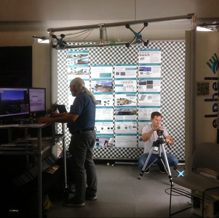
CVPR 2018 – from Elphel’s perspective
In this blog article we will recall the most interesting results of Elphel participation at CVPR 2018 Expo, the conversations we had with visitor’s at the booth, FAQs as well as unusual questions, and what we learned from it. In addition we will explain our current state of development as well as our near and far goals, and how the exhibition helps to achieve them.
The Expo lasted from June 19-21, and each day had it’s own focus and results, so this article is organized chronologically.
June 19, CVPR 2018, booth 132
While we are standing nervously at our booth, thinking: “Is there going to be any interest? Will people come, will they ask questions?”, the first poster session starts and a wave of visitors floods the exhibition floor. Our first guest at the booth spends 30 minutes, knowledgeably inquiring about Elphel’s long-range 3D technology and leaves his business card, saying that he is very impressed. This was a good start of a very busy day full of technical discussions. CVPR is the first exhibition we have participated in where we did not have any problems explaining our projects.
Q: Why does your camera have 4 lenses?
A: With 4 lenses we have 4 stereo-pairs: horizontal stereo-pair is responsible for vertical features (it is the same as in regular stereo-camera); the vertical pair detects horizontal features, while the 2 diagonal pairs ensure that almost any edge is detected. (Elphel Presentation, p.8).
A: Lidars are not capable of long range distance measurements. The practical maximum range of a lidar is 150-200 meters, while we target 500-2000 meters with a 150 mm stereo-base.(Elphel Presentation, p.7)
Q: How do you deal with thermal expansion?
A: there are 2 parts to this question: 1) thermal expansion of the calibrated lens is taken care of by the design of the sensor-lens module; 2) Thermal expansion of the whole camera is also an issue, especially with the larger stereo-base. The titanium tubes that form the cross of the X-Camera expand more on the “sunny side”, and the whole camera bends inward, like a flower. When taking images under the hot Utah sun, we had to wrap the tubes with insulation, covered in aluminum foil.
After some consideration we decided to remove the insulation wrapping for the CVPR show, because it makes the camera more presentable, and were surprised that this question came up so many times – we almost put the insulation cover back on.
Q: Do you build custom lenses?
A: We pre-select standard M12 lenses, because the quality of the lens can vary even within the same model. We have developed a full calibration process and post-processing software to compensate for optical aberrations, allowing to preserve the full sensor resolution over the camera FOV. Read more about aberration correction on Elphel blog.
Q: What is your part of the technology?
A: Everything: we have all parts: Hardware – cameras with aberration corrected lenses and thermally compensated sensor-lens module; a state of the art calibration facility and process; 3D-reconstruction software (Free Software, GNU GPL).
Q: What is the accuracy of your photogrammetry:
A: We comfortably work with 1/10 of a pixel.
Q: How dense is your 3D scene?
A: Currently: 324 x 242 overlapping tiles, with no dead zones.
Q: Does it build a 3D model in real-time?
A: Currently the 3D model is reconstructed in software in the post-processing of the acquired images. This software is tested for FPGA, with which we can achieve 12fps 3D-reconstruction on the camera. Our final goal is to design and manufacture custom ASIC with 3D processing on the chip. (Elphel Presentation, p.17)
The last visitor of the day from a large European company stopped at our booth around 6pm, 30 minutes before the end for the day, and we spend another hour talking and showing Elphel’s camera and high-resolution accurate images it produces. The lights on the floor went down, but we stayed and explain the technology behind our results and future plans. It was a nice day, well spent.
Day 2: Neural network focus.
End-to-End vs. Augmented
Our current results:- 500 meters, high resolution, 3D reconstruction with 5% accuracy with 150mm stereo-base (quad-stereo camera), passive (image-based)
- 2000 meters with 5% accuracy with 2 quad-stereo cameras based at 1256 mm from each other
- 3D-Reconstruction is done in post-processing with software simulated for FPGA porting. With FPGA – 12fps in 3D
Our near future goals:
- Train the neural network with the current 3D-image sets to achieve same results as in (2) – 2000 meter 3D reconstruction, with just one quad-sensor camera
- Port software to FPGA to achieve real-time 3D reconstruction (12 fps)
Our long-term goals:
- Manufacture custom ASIC for 3D-reconstruction to reconstruct 3D scenes on the fly with video frame rate. The small size of the custom chip will allow us to mass produce a long-range 3D reconstruction camera for industrial and commercial purposes. Smaller form-factor, inexpensive, and fast.
- Scalable design: a smaller stereo-base with 4 sensors – phone application (200 meter accurate 3D reconstruction for consumer applications); larger stereo-base: extremely long range passive 3D reconstruction – military applications, drone applications, etc.
Elphel’s approach to 3D reconstruction with the help of neural network is different from the mainstream one. This is partially due to our expertise is building calibrated hardware, which already produces robust 3D measurements. Therefore we see the value in pre-processing the images before feeding them to the NN similar to the eye pre-procesing visual information before sending it to the brain. The human eye receives 150 MPix of data, processes it on the retina, and sends only 1Mpix to the brain – 150 times reduction.
One question came up twice, both times from the conference attendees, about the difficulty the NN has to process high-resolution images. The current approach to NN training recommends to use low resolution raw images (640×480), because the NN has to be trained on a large amount of images (thousands). The last 6 slides of Elphel’s presentation talk about augmenting the NN with Elphel high-performance Tile Processor, that significantly reduces the amount of data, while leaving the “decision making” to the network.
We argue that the End-to-End approach is less efficient for high-resolution image processing then NN augmented with training-tree, linear image processing.
Elphel training sets for Neural Network:Elphel offers unique image sets for neural network training. These are high-resolution, space-invariant data sets.
Elphel is seeking collaboration with machine learning research teams working in the area of ML applications for 3D object classification, localization and tracking.
Day 3: Autonomous Vehicle Focus:
The exhibition is slowing down. Some booths start packing at midday. Elphel, however is busier than ever.
We have talked to about every self-driving car company that had it’s presence at CVPR. We also talked to other large corporations doing research in perception and 3D-reconstruction.
We start by visiting our neighbors – other exhibitors at the Expo, we are very curious what they develop, for which applications, can it be combined with our technology, can we learn something from them, and can they learn from us? It’s a collaborative spirit, with which we start conversation. One of our closest neighbors is Mapbox – an open source mapping platform for custom designed maps, so we start with them. We use Open street Map as well as other maps with our Scene Viewer for 3D-reconstructed scenes for locating scenes on the map as well as for the ground truth data. During lunch break at we add Mapbox tiles to our scene viewer. Mapbox exhibitors are pleased that it worked so well for us. Now they are also very interested in our technology!
Then we walk to other booths, learn about them and present Elphel.
Some of the responses we’ve got when we introduced our technology and our current results:
- Researcher from Apple: “You have the most unique technology on this Expo!”
- Autonomous Vehicle company A: “I can not believe you can accurately measure distances at 500 meters with just a small base of 150mm? With just 5-10% error? It is simply impossible! I have to come see it!” After visiting our booth seeing the demo he asks: “Can you demonstrate your technology on the car? It has to be in Singapore!”
- Autonomous Vehicle company B: ” We are happy with the use of the Lidars on the city streets, with close range perception and 30 mph driving speed. But on the highway, where the speed if much higher and the distance much farther the Lidar’s output is too sparse. Passive, long-range 3D reconstruction would be a perfect solution.”
- Autonomous Vehicle company C: “How dense is your 3D scene? Oh, it is dense, then we can use it.”
- Autonomous Vehicle company D: “We are building the perception solution for self-driving trucks. We need long-range distance measurement.”
- Autonomous Vehicle company E: “We have 16 different types of sensors on the car right now. I don’t think we have room to put another camera. Besides the area behind the wind shield is very valuable, we already have 4 cameras there – there is no room. By the way, we re-evaluate our approach every 6 months, and we just did that, so let’s, maybe, talk in 6 months again?”
Interesting thought – why would anyone need unobstructed windshield in a self-driving car? They did not explain that.
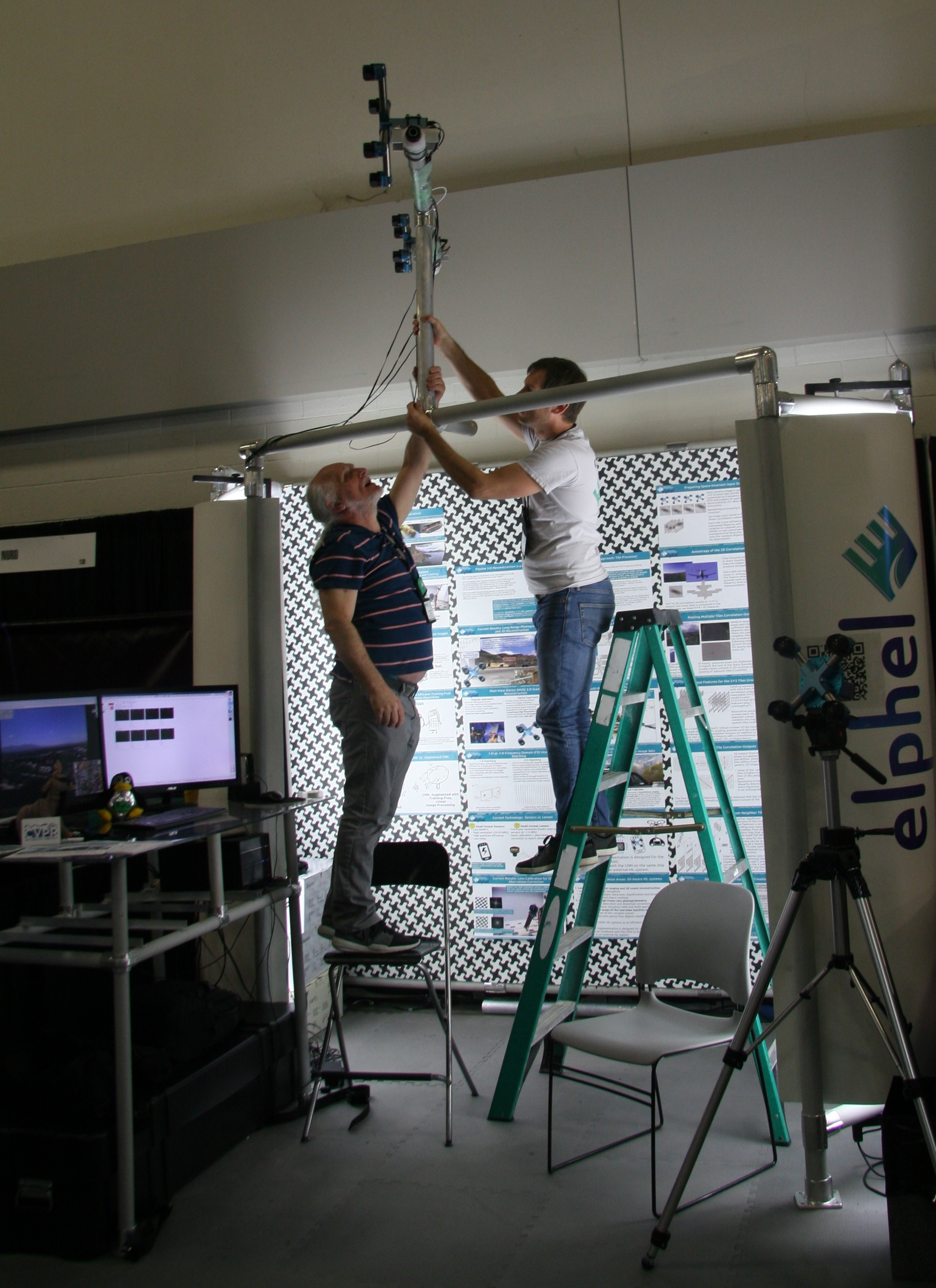
creating 3-D model of the CVPR 2018 Expo
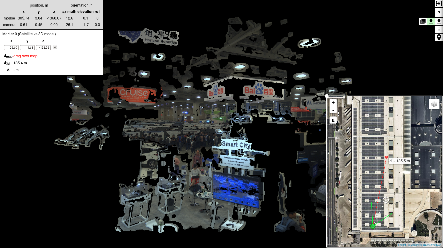
3D model view of CVPR 2018, made by Elphel 3D X-Camera
One last thing to do before the show is over is to get the 3D-X-Cam up high and build the 3D model of the CVPR 2018 EXPO in “real-time”!
Two Dimensional Phase Correlation as Neural Network Input for 3D Imaging
We uploaded an image set with 2D correlation data together with the import Python code for experiments with the neural networks and are now looking for collaboration with those who would love to apply their DL experience to the new kind of input data. More data will follow and we welcome feedback to make this data set more useful.
The application area we are interested in is an extremely long distance 3D scene reconstruction and ranging with the distance to baseline ratio of 1000:1 to 10,000:1 while preserving wide field of view. Earlier post describes aircraft distance and velocity measurements with up to 3,000:1 distance-to-baseline ratio and 60°(H)×45°(V) field of view.
Figure 1. Space-invariant 2D phase correlation data
Data set: source images, 2D correlation tiles, and X3D scene models
The data set contains 2D phase correlation output calculated from the 2592×1936 Bayer mosaic source images captured by the quad stereo camera, and Disparity Space Image (DSI) calculated from a pair of such cameras. Longer baseline provides higher range resolution and this DSI is serving as the ground truth for a single quad camera. The source images as well as all the used software is also provided under the GNU/GPLv3 license. DSI is organized as a 324×242 array – each sample is calculated from the corresponding 16×16 tile. Tiles are overlapping (as shown in Figure 3) with stride 8.
These data sets are provided together with the fully reconstructed X3D scene models, viewable in the browser (Wavefront OBJ files are also generated). The scene models are different from the raw DSI as the next software stages generate meshes, and that frequently leads to over-simplification of the original DSI (so most fronto parallel objects in the scene provide better range accuracy when probed near the bottom). Each scene is accompanied with the multi-layer TIFF file (*-DSI_COMBO.tiff) that allows to see the difference between the measured DSI and the one used in the rendered X3D model. File format and Python import software is documented in Oleg’s post “Reading quad stereo TIFF image stacks in Python and formatting data for TensorFlow”, the data files are directly viewable with ImageJ.
The first goal of applying neural network to this data is to improve DSI generation from the raw 2D correlation compared to what we can do now with the traditional code by using data from all correlation pairs and the neighbor tiles to propagate information along the objects edges and amplify correlation in low textured areas by pooling the correlation outputs from multiple tiles.
While there are no moving parts in the system, the overall process of measuring the DSI resembles human/animal stereo vision, where the eyes are converged for the expected object distance, and the visual processing deals with only a small residual mismatch, constantly adjusting the convergence. The difference here is that each tile can be individually “converged” for the requested disparity – this is done by combining integer pixel shift of the tile input window with the accurate fractional pixel shift by a phase rotator in the frequency domain to avoid any re-sampling errors. Currently prediction of the “convergence” (expected disparity) for the next tiles to measure is performed by a mixture of several algorithms (to avoid an expensive full disparity scan over the whole image). This process of predicting disparity is likely to be improved by a properly designed and trained network too, the one that will use the tile context.
As the current processing is recurrent (repeated “eye convergence” / mismatch processing), there are several options how to organize the training data. We decided to focus on sub-pixel matching, so for each scene with calculated ground truth DSI (from the dual camera rig) the correlation output is measured for the target disparity (convergence) in the range of minus 1 pixel to plus 1 pixel with the step of 0.1 pixel in the currently provided data sets. It makes total of 21 files of the correlation outputs. This partial disparity sweep around the ground truth is an alternative to a full disparity sweep that would require too much storage.
In addition to the raw Bayer images scene models have links to the JPEG images, corresponding to each sub-camera view. These images have aberrations corrected and they are partially rectified for the disparity = 0 (infinity). They are not rectilinear, and still have small radial distortion common to all of them, it is compensated during generation of the x3d models. The images have visible modulation caused by the Bayer mosaic – they were not subject to any (destructive) demosaic processing – only to the linear one. Each color channel is separately de-convolved with a set of space-variant kernels.
Figure 2. Dual quad camera rig
Available data seriesInitial data contains scenes captured with the car mounted dual quad camera rig (Figure 2) in two series:
- Salt Lake City State Street ↗
- Salt Lake City overlook (northern part of the city in the direction of the airport) ↗
The first series (80 scenes) was captured while driving north at a rate of 5 frames per second. Only the first four seconds (20 scenes) of each 20 second interval are posted to reduce the amount of uploaded data. The second series (59 scenes) was captured while standing and then slowly turning and starting to move.
More data will be added, we are open to suggestions – what data should be included to make the whole data set more useful. All available series combined are available at this link: ↗. Number of the scenes is definitely too small to extract the semantic information, but it may be enough to train the network to build DSI using small samples of the correlation tiles. At least to start with.
The frequently asked questions about this dataset Why is there a special format of the data set, why not just provide the raw images?We do provide raw Bayer images captured by the camera in JP4 format, but due to significant for the high-resolution images optical aberrations, complete end-to-end processing would require space-variant coefficients that to our understanding would require enormous resources and a very large number of images for training. Instead we propose to separate the space-variant pre-processing and provide space-invariant data to the network. And the 2D correlation data is the earliest space-invariant data available with this approach.
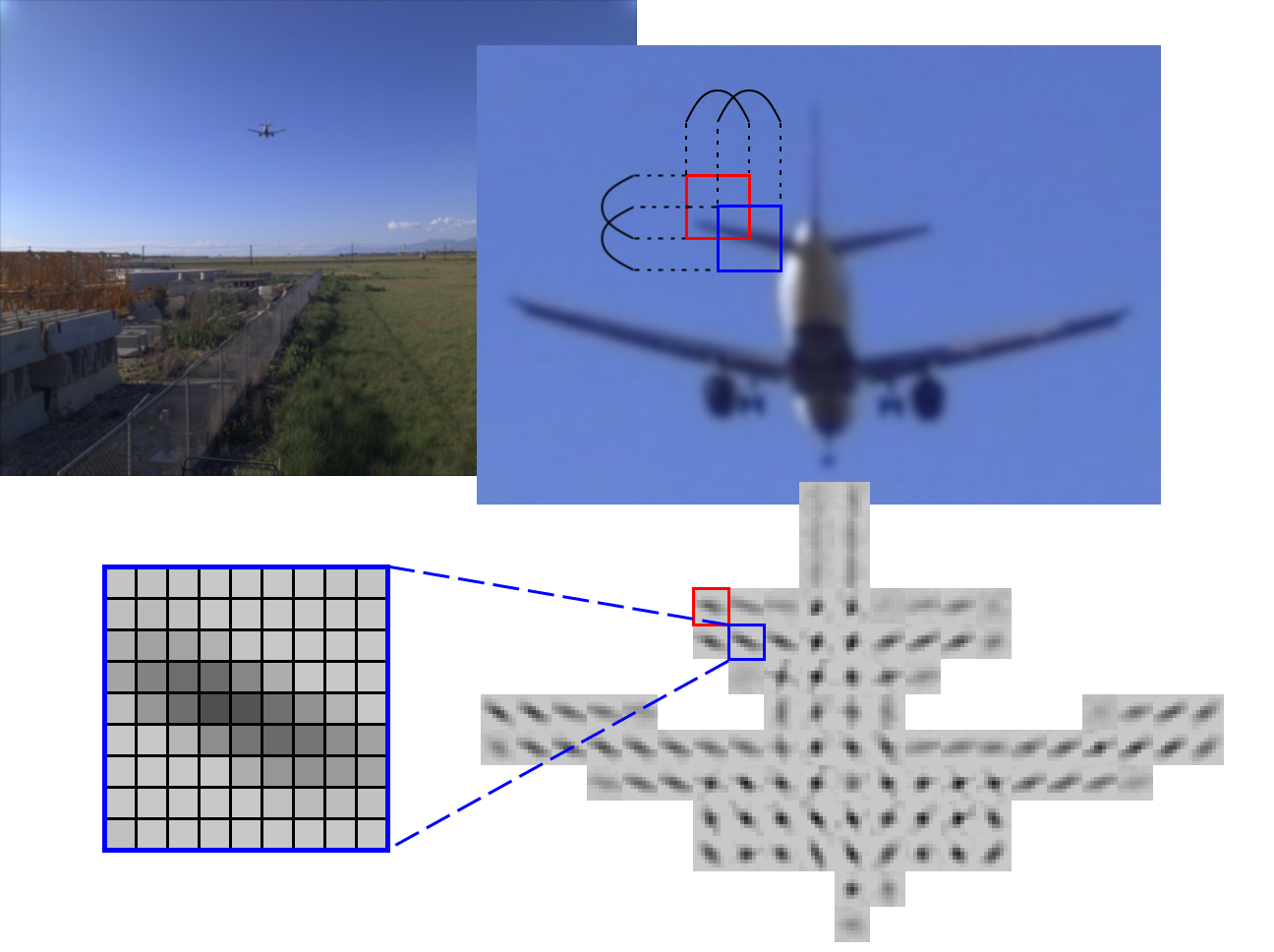
Figure 3. Anisotropy of the 2D correlation. Red and blue squares show two overlapping tiles in the source images and in the calculated 2D correlation.
Why do you use four cameras for stereo when most systems have just two?In the case when the source image contains nicely textured in all directions areas, the correlation output contains a sharp round spot and subpixel argmax calculation is not very difficult – polynomial interpolation provides good results. Unfortunately many real-life objects do not have convenient texture, and poor texture is Achilles’ heel of many vision-based 3D reconstruction systems. On the other hand discontinuity between foreground and background objects usually results in sharp edges that can be used for matching, and it is usually safe to assume that lack of visible features means that the surface is smooth and depth can be reconstructed by averaging over larger area. The edges may have any direction, but binocular systems with horizontal baselines are only sensitive to the vertical features. Figure 3. shows correlation output of a distant airplane where the correlation spots are stretched in the direction of the edges. The four-sensor camera in Figure 1 contains 6 pairs, and after combining horizontal and vertical there are 4 directions left, so for any edge direction there is a pair with a almost perpendicular to it.
Why don’t you use LIDARs for the ground truth data?Most available LIDARs have a rather short range of 150-250 meters, and we are interested in measuring larger scenes. So instead we decided to use a pair of similar quad cameras positioned at ~5 times larger distance than the quad camera baseline, so the measurements it provides are also 5 times more accurate and can be used for training as ground truth. Binocular system does have limitations as described above, so it will not provide accurate data for the horizontal features (like electrical wires so common over Salt Lake City).
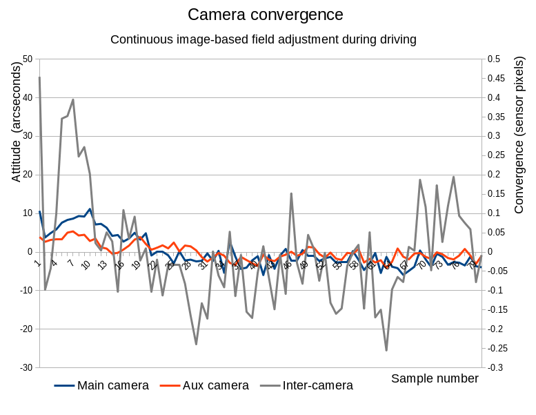
Figure 4. Field calibration results
What are the current limitations of the hardware?Individual quad cameras use precisely thermally compensated sensor front ends with the image plane movement relative to the sensor of less than ±0.02μ/°C, but the overall mount made of titanium tubes does bend when heated by the sun radiation from one side. Just few tenths of a pixel, but it is too much for the application, so until we have a new design we have to use field calibration and bundle-adjust individual sub-camera attitudes using the image data itself. It allows to keep misalignment to ~0.05 pix.
Dual camera rig (Figure 2) as currently implemented has its limitations that we temporarily mitigate with the field calibration. We are working on the rig improvements too – one of the mechanical issues is that when driving at freeway speeds we noticed 55 Hz torsion oscillations (two cameras rotating in opposite directions at the ends of the 1.5 m aluminum tube) of 0.4 pix amplitude. So until we will strengthen the rig we had to limit data set to the images captured at lower speeds to keep vibration-caused mismatch under 0.1 pix.
Figure 4. shows results of the field calibration for the image series captured during driving along the State Street. Each quad camera (main with the 258 mm baseline and auxiliary with the 150 mm one) had adjusted its sensor front end attitude angles using the image data, same with the attitude of the auxiliary camera as a whole with respect to the main one (baseline of 1256 mm). The results of the distance measurements obtained from this long baseline pair were then used as ground truth for the individual quad cameras. Relatively strong correction required for the first ~20 samples was caused by the changing temperature in the camera connection tubes after slowing down from the freeway speed to the city one.
Electronic rolling shutter (ERS) limitations. We really love small format high-resolution image sensors perfected by the cellphone industry for the image quality and sensitivity, but that performance currently requires Electronic Rolling Shutter (ERS) that leads to image distortions of the moving objects (or caused by the moving/rotating camera itself). In the presence of movement of the objects (or camera egomotion) the measured disparity depends on the time difference between the moments the same feature is captured by the sub-cameras. The sensors are mechanically aligned to be parallel within 5 pixels that corresponds to 0.2ms of the readout time. That means that horizontal pairs capture all objects almost simultaneously regardless of disparity, for the vertical and diagonal pairs that time difference increases proportionally to the disparity, but for the far objects (where disparity accuracy is most important) that difference is still small (0.03ms for each disparity pixel). Currently posted image sets do not have any ERS correction, and that somewhat deteriorates performance for the near objects, but when considering just the egomotion (both translation and rotation) this effect can be easily compensated, at least for the uniform rotation on movement.
In the posted image set ERS is not an issue for small (<5 pix) disparities, we will add software compensation over the full disparity range of the scenes for uniform movements, and later will use IMU to compensate higher frequency movements also.
Reading quad stereo TIFF image stacks in Python and formatting data for TensorFlow
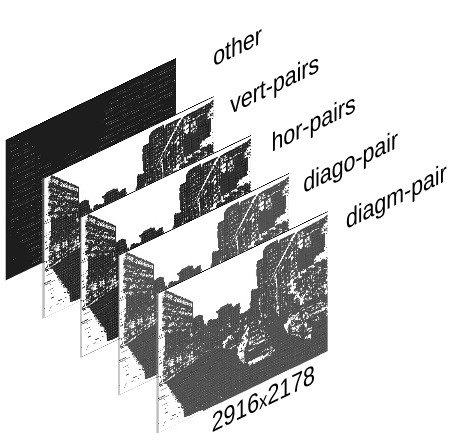
Fig.1 TIFF image stack
The input is a <filename>.tiff – a TIFF image stack generated by ImageJ Java plugin (using bioformats) with Elphel-specific information in ImageJ written TIFF tags.
Reading and formatting image data for the Tensorflow can be split into the following subtasks:
- convert a TIFF image stack into a NumPy array
- extract information from the TIFF header tags
- reshape/perform a few array manipulations based on the information from the tags.
To do this we have created a few Python scripts (see python3-imagej-tiff: imagej_tiff.py) that use Pillow, Numpy, Matplotlib, etc..
Usage:
~$ python3 imagej_tiff.py <filename>.tiff
It will print header info in the terminal and display the layers (and decoded values) using Matplotlib.
Subtasks 1. and 2. are simply done by Pillow. As for 3., if it was a simple TIFF image stack there would be no need to have extra scripts.
If the layer were just stacked along depth the shape would be (2178, 2916, 5). The script reshapes the data into tiles and puts the values into a separate array, so the output is 2 Numpy arrays:
- image data shape: (242, 324, 9, 9, 4) with the layers along the last dimension
- values data shape: (242, 324, 3)
And they are ready to be used in the Tensorflow.
For more details and example output, see this wiki page or inspect the source. The most detailed general info is probably in the slides from our presentation for CVPR2018 – format description starts from p.19.
File samplesActual files can be found here or go to 3d+biquad, open individual models and hit the light green button to ‘Download source files for ml’.
Without using Python displaying layers and decoding tags is natively supported by ImageJ or Fiji. To read the tags exiftool or tiffinfo linux programs can be used.
Other librariesOther Python libraries that could have worked (but examples for Pillow were easier to find):
Elphel at CVPR 2018
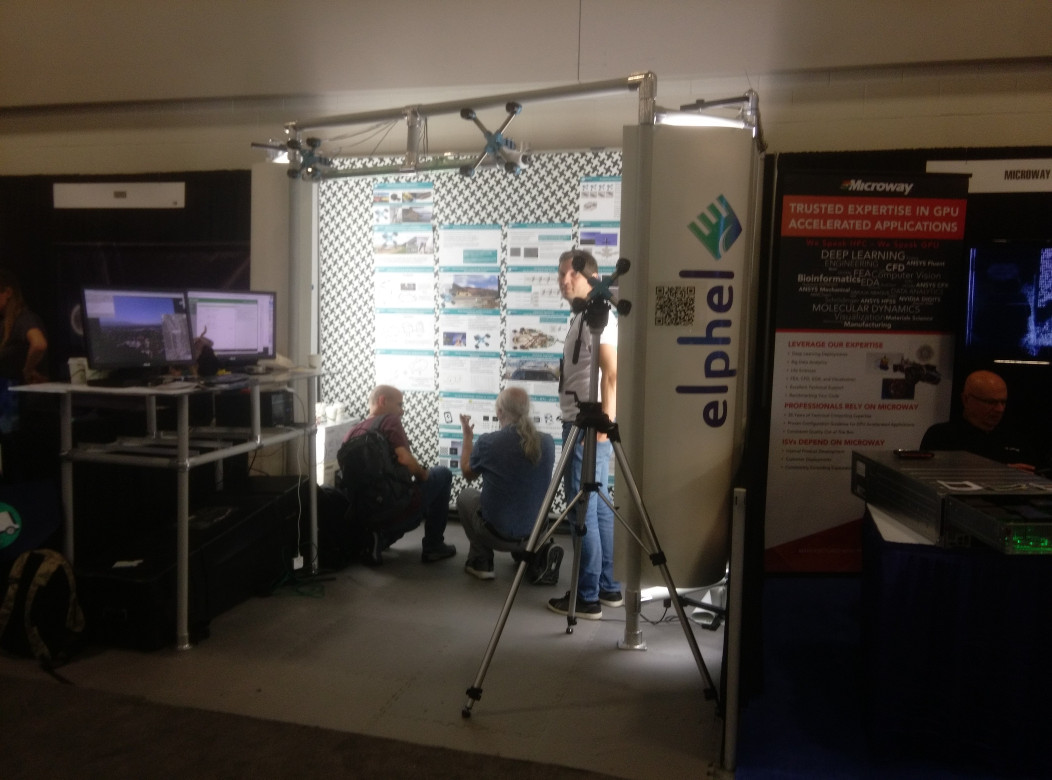
Elphel booth at CVPR 2018 Expo
Elphel is presenting at CVPR 2018 EXPO: Long Range Passive 3D Reconstruction System, providing NN with custom training sets, enabling realtime 3D-aware machine learning systems.
Please visit us at CVPR, Booth 132.
You can also find our presentation and related articles on wiki page https://wiki.elphel.com/wiki/CVPR2018
Capturing Aircraft Position with the Long Range Quad Stereo Camera
Figure 1. Aircraft positions during descent captured with the quad stereo camera. Each animation frame corresponds to the available 3-D model.
While we continue to work on the multi-sensor stereo camera hardware (we plan to double the number of sensors to capture single-exposure HDR image sets) and develop code to get the ground truth data for the CNN training, we had some fun testing the camera for capturing aircraft position in 3-D space. Completely passive method, of course.
We found a suitable spot about 2.5 km from the beginning of the runway 34L of the Salt Lake City international airport (exact location is shown in the model viewer) so approaching aircraft would pass almost over our heads. With the 60°(H)×45°(V) field of view of the camera aircraft are visible when they are 270 m away horizontally.
Camera was set to capture synchronized image sets at 5 frames per second (same as in Fig. 1 animation), each set was processed independently without any relation to the other ones (no optical flow or motion vectors). Our existing (not airplane-aware) prototype software generated the scene 3-D models, they in turn were used to measure the aircraft positions. Result accuracy may be improved by using directly the intermediate Disparity Space Image (DSI) data – current reconstruction code tries to fit some flat surfaces to approximate the DSI data. At long distances there is insufficient data about the shape of the objects, so at ~500 m range (Fig. 2) the software used a fronto-parallel surface (distances to the aircraft nose, center, and tail are the same) and at ~600m it selected a tilted surface in the wrong direction, so the measured distance to the tail is larger than the one measured to the nose and center.
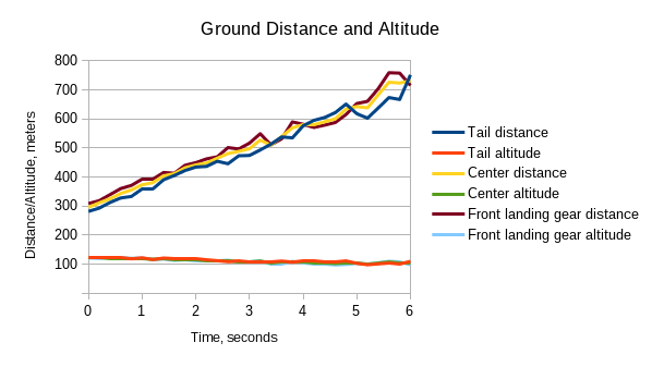
Figure 2. Ground distance and altitude of the three points sampled.
The measurements accuracy is still good, considering that the disparity of 1 image pixel corresponds for this short baseline camera to 527 meters range, at 800 m 1/10 pixel disparity precision corresponds to 120 m uncertainty. Ground speed and the descend rate (indicated in the animation) are calculated between the first captured set and the current one, so the last value averages over the full 6 seconds.
This method of capturing aircraft position and speed does not require that it travels directly to/from the camera, it can fly in any direction. There could also be multiple aircraft (such as UAVs) in the same camera view. Another 3-D scene (Fig. 3) captured from the same spot perpendicular to the flight direction shows an aircraft at 1600 m from the camera at 110 m altitude. According to the map the center line of the 34R runway is 14% farther (at 1820 m) from the camera position. That corresponds to 0.045 pix disparity error in the distance measurement, so calculated ground speed and altitude would also be 14% lower than actual.
Figure 3. Aircraft traveling perpendicular to the view direction.
Each of the provided 3-D scene models has the corresponding “set of 4 images” link on the settings page that can be viewed as an animation, manually iterated over or downloaded – the one for Fig. 3 scene shows how a 0.33 pixel wiggle of the FedEx MD-11 image looks like (images are zoomable and pannable). Here are the direct links for image sets of the first (1.75 pix disparity) and the last (0.7 pix disparity) of the scene models of the approaching B737 shown in Fig. 1.
These four images are not used in the actual reconstruction process, they are rendered from the source raw (JP4 format) ones for the specified disparity (D0.0 in the file names show that disparity was 0.0 pixels) for viewing or evaluating with alternative software. These images are not rectilinear and have residual common (for all four) radial distortion. They have optical aberrations corrected by the space-variant deconvolution, sub-camera residual misalignment is field-corrected (such misalignment may be caused by an uneven heating of the camera tubular structure by the direct sunlight). The images are partially rectified to the common radial distortion model that bests fits simultaneously all four sub-cameras. The remaining radial distortion is compensated during final generation of the 3-D model. These images have visible grid artifacts caused by the Bayer pattern – no de-mosaic processing is involved because it hurts linear operations over the images, and it is not adequate for the peripheral image areas (see earlier post). Each color component is processed separately for the phase correlation, when combining texture images these artifacts are reduced as they are not coherent between the channels. Any additional non-linear improvements of the Bayer mosaic suppression can be applied to the texture generation step, not to the data used for correlation.
Implementing a linux driver for an image sensor for NC393
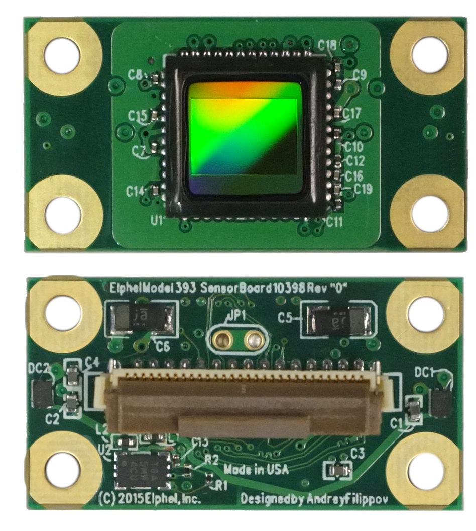
Fig.1 MT9F002
MT9F002This post briefly covers implementation of a driver for On Semi’s MT9F002 14MPx image sensor for 10393 system boards – the steps are more or less general. The driver is included in the latest software/firmware image (20180416). The implemented features are programmable:
- window size
- horizontal & vertical mirror
- color gains
- exposure
- fps and trigger-synced ports
- frame-based commands sequence allowing to change settings of any image up to 16 frames ahead (didn’t need to be implemented as it’s the common part of the driver for all sensors)
- auto cable phase adjustment during init for cables of various lengths
- Get the register reference document for MT9F002
- Setup the Eclipse IDE for linux kernel development – see instructions
Capturing images without the driver
There is a set of scripts used for verification in software (on PC) and hardware (on the target board). Among other things they can be used to establish initial communication with a sensor, run registers initialization and acquire the first images. The process for MT9F002 is described on our wiki.
In general the driver can be split into 2 parts:
- common for all sensors – sets up working with fpga frame-based command sequencers (see NC393 development progress and the future plans).
- sensor specific – commands that do actual communication with a sensor. This is the part needs to be implemented.
For a sensor there are a few tables and a few functions, the most important ones are:
tables:
- mt9f002_pages – a ‘page’ is the upper byte of a 16-bit register address of the sensor (for 8-bit reg addresses the page number is 0x00), the table should list all available pages in the sensor – or at least the most important ones – they are used to program fpga’s 256-max records per port tables used to write commands and at least one record is used to read from port – so in general for a setup w/o a MUX board the limit of allowed pages per sensor is 256-1 = 255 (with a MUX + 3x sensors on a single port it is 256-2(mux write & read)-4(3x sensor read + 1x broadcast read))/4 = 62)
- mt9f002_par2addr – used convert 256 8-bit parameters available as P_SENSOR_REGSxxx to 16-bit register address
- mt9f002_ahead_tab – sequencer commands latencies – leave default, they are needed on the final stages of development
functions (they are registered on top of the common ones):
- mt9f002_pgm_detectsensor – remove reset read sensor id
- mt9f002_pgm_initsensor – init registers that select interface, sensor’s PLL multipliers/dividers and other required settings
- mt9f002_pgm_exposure – program exposure
- mt9f002_pgm_window – program image width and height
- mt9f002_pgm_limitfps – limit fps based on compressor capabilities and trigger period settings
- mt9f002_pgm_gains – program color gains
- mt9f002_pgm_triggermode – set sensor in triggered mode
- mt9f002_pgm_sensorregs – write sensor registers directly
See this article for more details.
Dual Quad-Camera Rig for Capturing Image Sets
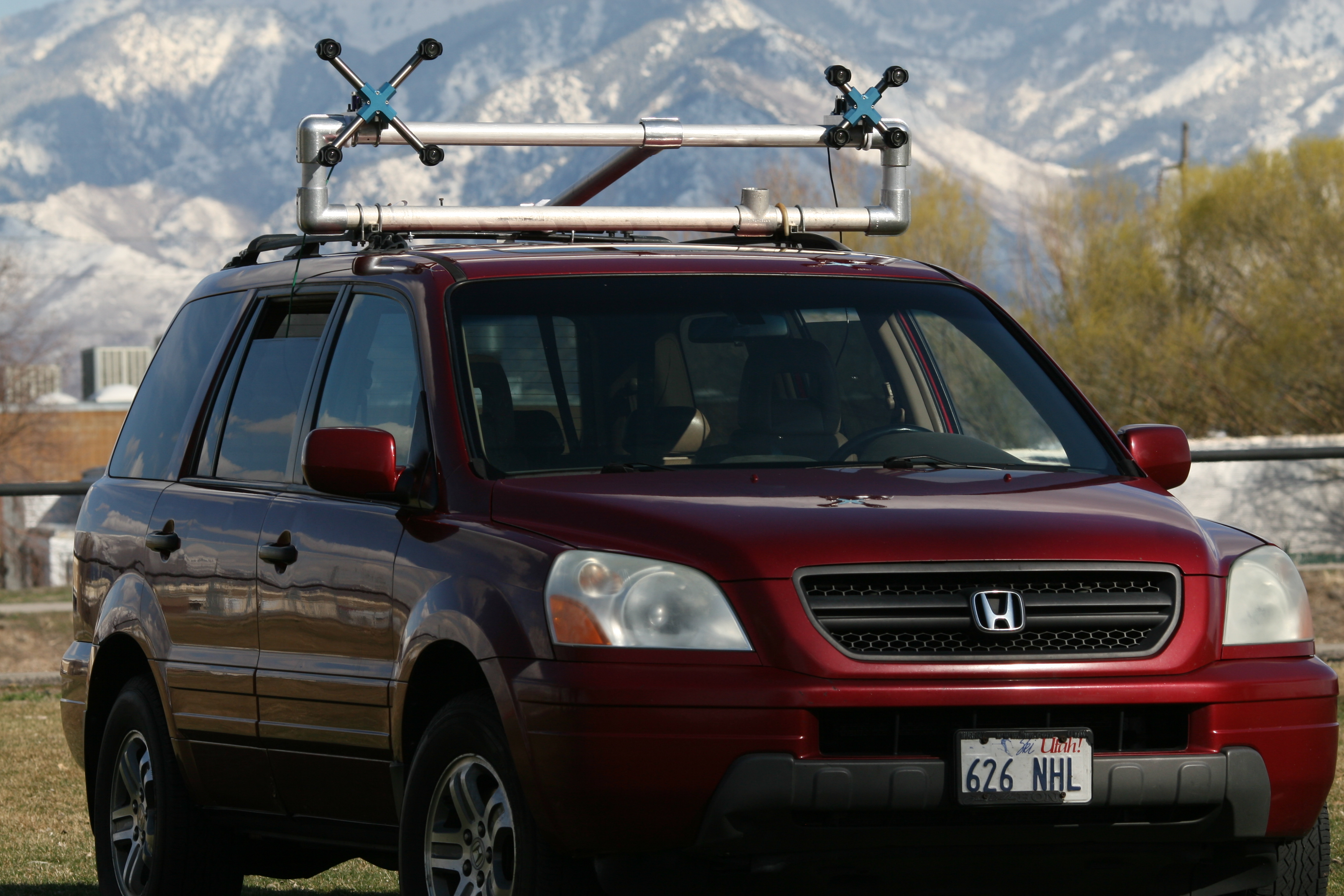
Figure 1. Dual quad-camera rig mounted on a car
Following the plan laid out in the earlier post we’ve built a camera rig for capturing training/testing image sets. The rig consists of the two quad cameras as shown in Figure 1. Four identical Sensor Front Ends (SFE) 10338E of each camera use 5 MPix MT9P006 image sensors, we will upgrade the cameras to 18 MPix SFE later this year, the circuit boards 103981 are in production now.
We decided to use cameras with different baselines: 150 mm and 258 mm, the distance between the quad-camera centers is 1256 mm. The distance map calculated from the larger of the two cameras will have higher precision, than the distance map from the smaller one. For the same processing algorithms and the same object the distance resolution is reverse proportional to the baseline. Even higher resolution will be achieved by fusing depth maps from the two cameras together. The higher precision results may be used for the cost functions of the lower distance resolution camera instead of the unavailable real ground truth data. To make the rig sufficiently rigid the cameras are mounted on the aluminum tube (OD=57 mm), and that tube is attached to the rest of the mount through the vibration isolators.
Each of the two cameras uses matched set of the lenses with focal length variation of less than 1% to simplify frequency domain mutual image rectification. Cameras still need fine alignment and calibration, after that we will start image sets capturing.
This year Computer Vision and Pattern Recognition conference (CVPR 2018) will be held in Salt Lake City, Utah. We plan to participate in the CVPR exhibition and we will be happy to see visitors at Elphel office that is less than 10 km from the conference venue.
High Resolution Multi-Vew Stereo: Tile Processor and Convolutional Neural Network
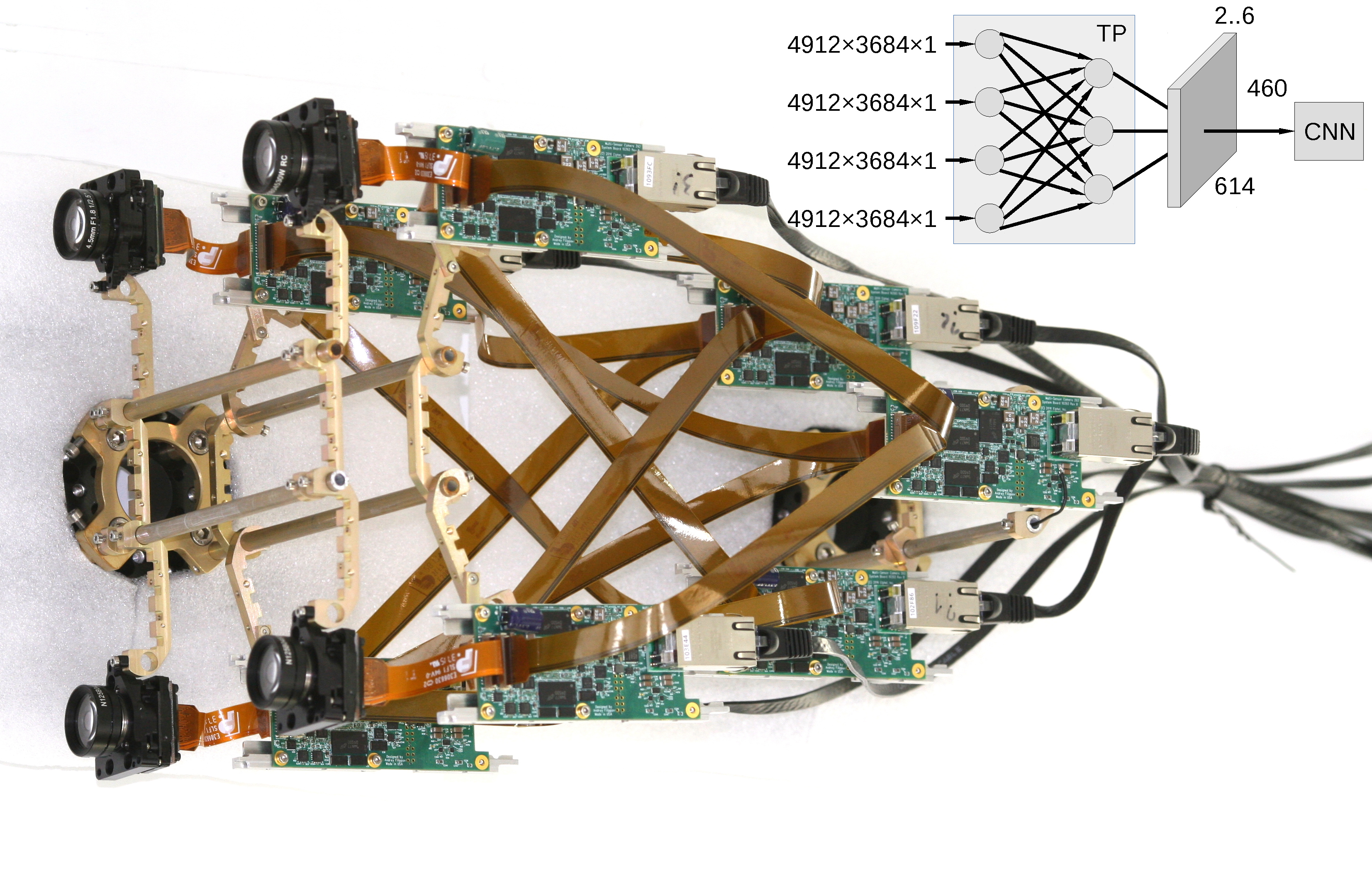
Figure 1. Multi-board setup for the TP+CNN prototype
This article describes our next steps that will continue the year-long research on high resolution multi-view stereo for long distance ranging and 3D reconstruction. We plan to fuse the methods of high resolution images calibration and processing, already emulated functionality of the Tile Processor (TP), developed RTL code for its implementation and the Convolutional Neural Network (CNN). Compared to the CNN alone this approach promises over a hundred times reduction in the number of input features without sacrificing universality of the end-to-end processing. The TP part of the system is responsible for the high resolution aspects of the image acquisition (such as optical aberrations correction and image rectification), preserves deep sub-pixel super-resolution using efficient implementation of the 2-D linear transforms. Tile processor is independent of any training, only a few hyperparameters define its operation, all the application-specific processing and “decision making” is delegated to the CNN.
Machine Learning for 3D Scene ReconstructionMachine learning is an active development area, and its applications to the 3D scene reconstruction stimulated by the autonomous vehicles including self-driving cars is no exception. Use of the CNNs to extract surfaces from the random-dot stereograms was published as early as 1992[1]. Most of the modern researches use standard image sets: Middlebury stereo data set[2] for high resolution near objects and KITTI[3] for the longer range applications. KITTI images are acquired from a moving car, they have attached ground truth data captured by the LIDAR. This image set uses binocular pairs and has relatively low resolution (1.4 MPix) compared to the modern image sensors, and still most of the CNN architectures require from seconds to thousands of seconds even when implemented with GPU devices and so are not yet suitable for the real-time applications.
Most of the CNNs[4] input raw pixel data and perform unary feature extraction in the parallel (one for each image in a stereo set) subnets, merge features and perform additional processing of the resulting 3d data. This is a so-called “siamese” network architecture that benefits from sharing parameters between the identical subnetworks. It is common to put most resources to the unary part of the processing resulting in truncating of the common stage of the processing that can consist of just a single layer(Fast Architecture in [4]). Efficient implementation in [5] limits CNN processing to just generate DSI and use traditional methods of DSI enhancement such as semi-global matching [6], other architectures split network after exchanging features and generate depth maps for each of the stereo images individually[7].
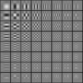
Figure 2. 2D MDCT basis functions (¼ of all MCLT ones for N=8)
Convolutional Neural Networks and the Frequency Domain ProcessingEarly layers of the various CNNs (and the eye retina too) are very general and even remind the basis functions (Figure 2) of the two-dimensional Fourier (DFT), cosine/sine (DCT and DST) and wavelet (DWT) transforms so it is no surprise that there are works that explore combinations of such transforms and the neural networks. Some of them [8, 9] exploit energy concentration property of these transforms that makes possible popular image compression such as JPEG. Others [10, 11] evaluate efficiency of the available Fast Fourier Transform implementations to speed-up convolutions by converting image data to the frequency domain and then applying the pointwise multiplication according to the convolution-multiplication property. Improvement is modest, as the frequency domain calculations are most efficient for the large windows, while most modern CNNs use small ones, such as 3×3, where Winograd algorithm is more efficient.
Tile Processor and the High Resolution Multi-View CameraMulti-view high resolution cameras present a special case where frequency domain processing results may lead to the reduction of the CNN input features by two orders of magnitude compared to raw pixel input. As described in the earlier post Tile Processor is using efficient Modulated Complex Lapped Transform (MCLT) conversion of the Bayer mosaic (color) high resolution image data to the frequency domain, simultaneously providing subpixel resolution shift for image rectification. Frequency domain processing includes space-variant optical aberration correction (required for the high resolution small format image sensors), phase correlation for image pairs and textures processing if it is required in addition to the distance (disparity) measurement. After channels/pairs merging the frequency domain data is converted back to the pixel domain where the tile correlation maximums are located and measured. Each overlapping tile is 16×16 pixels, the tile period (corresponding to stride in CNN terms) is 8×8 pixels. In the case when only the disparity value and confidence are output from each tile it makes 2 features. If the raw pixels were input, for 4 channels it would be 4*8*8 = 256 features or 128 times more. It may be useful to increase the number of features and supplement average disparity for all 4 pairs of quad camera with separate and horizontal and vertical pairs to improve foreground-background separation, in that case the feature reduction would still be over 40.
Conversion of the raw pixels to the Disparity Space Image (DSI) involves significant reduction of the (X,Y) resolution, when using four of the 18 MPix (4912×3684) imagers the DSI resolution is just 614×460, – isn’t it a waste of the sensor resolution? No, it is not:
- a deep sub-pixel resolution for disparity measurement needed for long-distance ranging requires matching of the large image areas anyway
- most of the image area for the most real-world images corresponds to smooth 3-d surfaces where assumption of a common disparity value for a tile is reasonable.
- the initial image resolution is preserved by the TP when source images are converted to the textures (simultaneously improving quality as the data from 4 rectified images is averaged)
- pixel-accurate distance map may be restored by extra processing the pixel data for selected tiles where depth discontinuity is detected, then assigning each pixel to one of the available surfaces.
Significant (42..128) reduction of the input features is not the only advantage of the TP+CNN combination over the CNN alone. Being “convolutional” CNNs depend on translation symmetry, the groups of related pixels are treated the same way regardless of their localization in the image. That is only an approximation, especially when dealing with the high resolution images and extracting subpixel disparity values. This divergence from the strict convolution model is caused by the optical aberrations and distortions and requires use of the space-variant convolution instead, or performing complete aberration correction and image rectification before the images are fed to the network. Otherwise both the complexity of the network and amount of training data would increase dramatically. Image rectification with pixel (or slightly better) precision is a common task in stereo processing. It involves interpolation and re-sampling of the pixel data, the process that leads to the phase noise introduction, especially harmful when deep super-resolution of the matched images is required. Tile processor implementation combines multiple operations (fractional pixel image shifts, optical aberrations correction, phase correlation of the matched pairs), TP avoids image re-sampling from the sensor pixel grid by replacing it with the phase rotation in the frequency domain.
Final step that reduces the number of features that are sent from the TP to the CNN is extraction of the disparity value by calculation of the argmax of the phase correlation data. This function has to be calculated with subpixel resolution for the data defined on the integer pixel grid. Certain biases are possible, and the TP implementation offers trade-off between speed and accuracy. The result disparity value is a sum of the pre-applied disparity (implemented as a phase rotation in the frequency domain on top of the integer pixel shift) and the argmax value (correlation maximum offset from zero). When higher accuracy is required, a second iteration may be performed by applying the full disparity from the first iteration, then the residual argmax offset will be close to zero and less subject to bias.
System Performance Estimation and the Prototype SetupOptimal system for the real-time high resolution 3-D scene reconstruction and ranging would require development of the application-specific SoC. If used with a set of four 18 MPix image sensors (such as ON Semiconductor AR1820HS) and a single ×16 1600 MHz DDR4 memory device, the 16 nm technology process, the TP subsystem will be capable of 10 Hz operation covering the full 4912×3684 frames reserving half of the memory bandwidth for other then TP operations.
We plan to emulate such system using available NC393 camera electronic and optical-mechanical components, including multiple 10393 system boards based on Xilinx Zynq 7030 SoC. Each such board has a GigE port and four identical sensor ports routed directly to the FPGA I/O pads allowing flexible assignment of pin functions. Typical applications include up to 8 differential LVDS pairs, clock pair, I²C and clock input. The same connectors can be used for high-speed communication between the 10393 boards. Partitioning the system into multiple boards will allow to fit the required TP functionality into smaller FPGAs, then send the result features (614×460×6) over the GigE to a workstation with GPU for the experiments with different CNN implementations. The system bandwidth will be lower than that of the application-specific SoC, the 10 Hz operation will be possible with 5 MPix sensors (2.5 Hz with 18 MPix).
Inter-board connections are shown in Figure 1 (just the connections, the actual prototype camera will look more like in Figure 3, but with a wider body). Five to seven of the 10393 boards are arranged in 2 layers. Four layer 1 boards use one of the sensor ports to receive image data from the attached sensor, perform image conditioning, flat-field correction and store data in the dedicated DDR3 memory. They later read the data as 16×16 pixels overlapping tiles, calculate the tile centers using calibration data and requested location and nominal disparity from the data received over the GigE. Each tile is transformed to the frequency domain, the data is subject to the space-variant aberration correction. The result frequency domain tiles are output through three remaining sensor ports that are reconfigured to be LVDS transmitters. The layer 2 boards simultaneously receive frequency domain data through all 4 of their sensor ports from the layer 1 and perform phase correlation (pointwise multiplication followed by normalization) on the image pairs. There could be just a single layer 2 board, or up to 3 (limited by the available layer 1 ports) to perform different types of correlations in parallel (all 4 pairs combined, two vertical pairs and separately 2 horizontal pairs for better foreground/background separation. The results of the frequency domain calculations are then transformed to the pixel domain and the argmax is calculated. Then argmax value is used to calculate the full tile disparity, and the corresponding correlation value – as a disparity confidence. The pair (disparity, confidence) for each tile is then sent over GigE to the CNN implemented on a workstation computer.
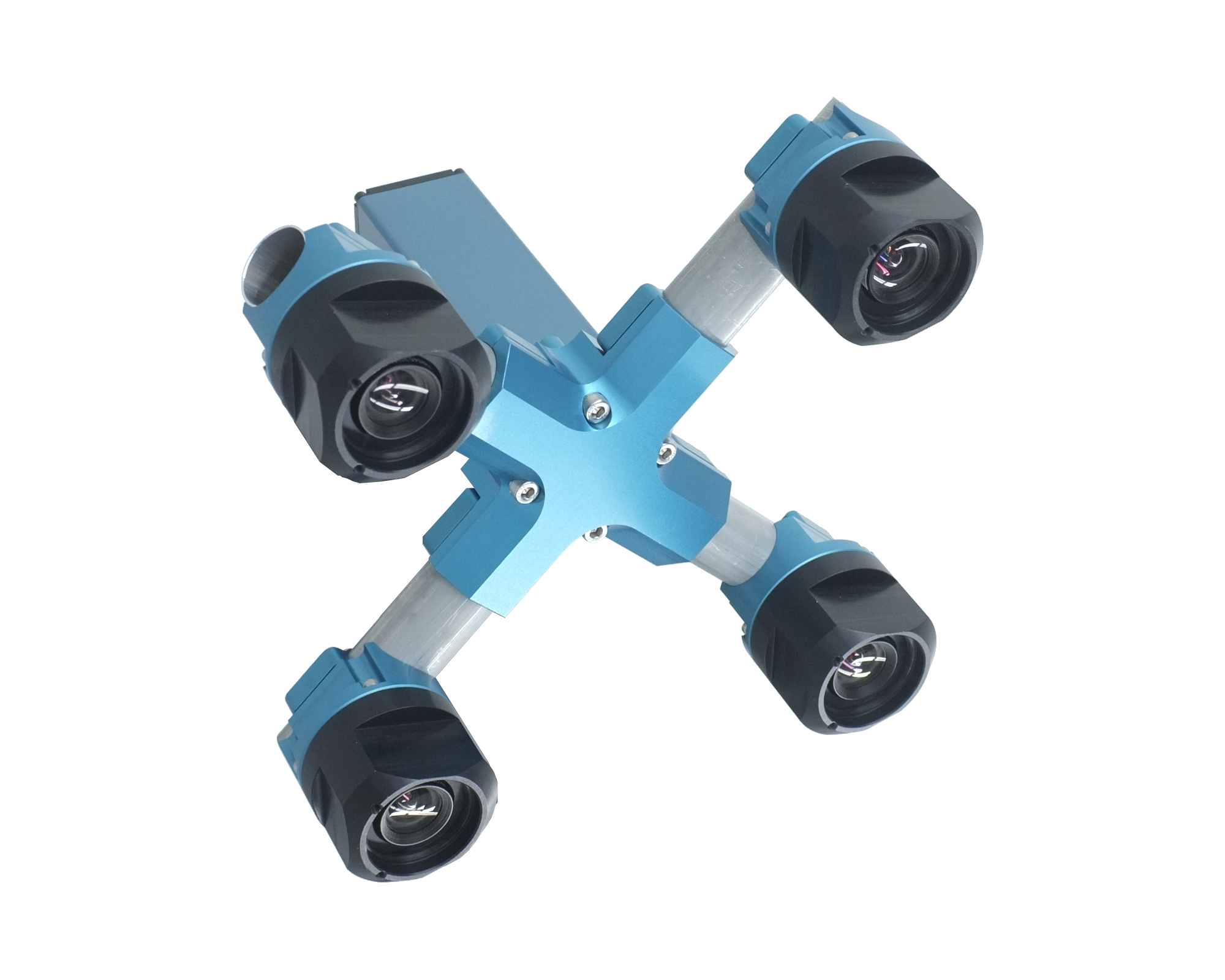
Figure 3. Quad sensor camera for image sets acquisition
Image Sets for Training and TestingWhile the TP functionality is already tested with the software emulation, and the efficient implementation is developed, more research is needed for the CNN part of the system. Available image sets, such as KITTI[3] have insufficient resolution (1.4 MPix) and they use different spatial arrangement of the cameras. We plan to capture high resolution quad camera image sets using available NC393-based cameras that will be upgraded from 5 MPix to 18 MPix sensors of the same 1/2.3″ format so the optical-mechanical design will remain the same. As we are primarily interested in long distance ranging (few hundreds to thousands meters), use of the LIDARs to capture ground truth data is not practical. Instead we plan to mount a pair of identical quad cameras (with the baseline of 150mm) on a car 1500 mm apart, pointed in the same direction, so when the 3D measurements from these quad cameras are fused, the accuracy of the composite distance data would be ten times better, because the effective baseline will be 1500mm. Of course that method has some limitations (it will not help to improve data from the poorly textured objects) but it will provide higher absolute distance resolution that can be used for the loss function during CNN training. Data from the individual quad cameras will be used for training and testing of the network.
All acquired images, related calibration data and software will be available online under GNU GPL.
References[1] Becker, Suzanna, and Geoffrey E. Hinton. “Self-organizing neural network that discovers surfaces in random-dot stereograms.” Nature 355.6356 (1992): 161.
[2] Scharstein, Daniel, et al. “High-resolution stereo datasets with subpixel-accurate ground truth.” German Conference on Pattern Recognition. Springer, Cham, 2014.
[3] Menze, Moritz, and Andreas Geiger. “Object scene flow for autonomous vehicles.” Proceedings of the IEEE Conference on Computer Vision and Pattern Recognition. 2015.
[4] J. Zbontar and Y. LeCun, “Stereo matching by training a convolutional neural network to compare image patches,” Journal of Machine Learning Research, vol. 17, no. 1-32, p. 2, 2016.
[5] W. Luo, A. G. Schwing, and R. Urtasun, “Efficient deep learning for stereo matching,” in Proceedings of the IEEE Conference on Computer Vision and Pattern Recognition, pp. 5695–5703, 2016.
[6] H. Hirschmuller, “Accurate and efficient stereo processing by semi-global matching and mutual information,” in Computer Vision and Pattern Recognition, 2005. CVPR 2005. IEEE Computer Society Conference on, vol. 2, pp. 807–814, IEEE, 2005.
[7] J A. Kendall, H. Martirosyan, S. Dasgupta, P. Henry, R. Kennedy, A. Bachrach, and A. Bry, “End-to-end learning of geometry and context for deep stereo regression,” arXiv preprint arXiv:1703.04309, 2017.
[8] Sihag, Saurabh, and Pranab Kumar Dutta. “Faster method for Deep Belief Network based Object classification using DWT.” arXiv preprint arXiv:1511.06276 (2015).
[9] Ulicny, Matej, and Rozenn Dahyot. “On using CNN with DCT based Image Data.” Proceedings of the 19th Irish Machine Vision and Image Processing conference IMVIP 2017
[10] Vasilache, Nicolas, et al. “Fast convolutional nets with fbfft: A GPU performance evaluation.” arXiv preprint arXiv:1412.7580 (2014).
[11] Lavin, Andrew, and Scott Gray. “Fast algorithms for convolutional neural networks.” Proceedings of the IEEE Conference on Computer Vision and Pattern Recognition. 2016.
Photo Finish
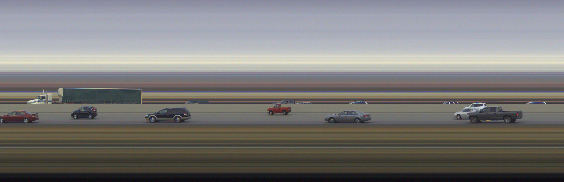
Since 2005 and the older 333 model, Elphel cameras have a Photo Finish mode. First, it was ported to 353 generation, and then from 353 to 393 camera systems.
In this mode the camera samples scan lines and delivers composite images as video frames. Due to the Bayer pattern of the sensor the minimal sample height is 2 lines. The max fps for the minimal sample height is 2300 line pairs per second. The max width of a composite frame can be up to 16384px (is determined by WOI_HEIGHT). A sequence of these frames can be simply joined together without any missing scan lines.
Current firmware (20180130) includes a photo finish demo: http://192.168.0.9/photofinish.
A couple notes for 393 photo finish implementation:
- works in JP4 format (COLOR=5). Because in this format demosaicing is not done it does not require extra scan lines, which simplified fpga’s logic.
- fps is controlled:
- by exposure for the sensor in the freerun mode (TRIG=0, delivers max fps possible)
- by external or internal trigger period for the sensor in the snapshot mode (TRIG=4, a bit lower fps than in freerun)
See our wiki’s Photo-finish article for instructions and examples.
Efficient Complex Lapped Transform Implementation for the Space-Variant Frequency Domain Calculations of the Bayer Mosaic Color Images
This post continues discussion of the small tile space-variant frequency domain (FD) image processing in the camera, it demonstrates that modulated complex lapped transform (MCLT) of the Bayer mosaic color images requires almost 3 times less computational resources than that of the full RGB color data.
“Small Tile” and “Space Variant”Why “small tile“? Most camera images have short (up to few pixels) correlation/mutual information span related to the acquisition system properties – optical aberrations cause a single scene object point influence a small area of the sensor pixels. When matching multiple images increase of the window size reduces the lateral (x,y) resolution, so many of the 3d reconstruction algorithms do not use any windows at all, and process every pixel individually. Other limitation on the window size comes from the fact that FD conversions (Fourier and similar) in Cartesian coordinates are shift-invariant, but are sensitive to scale and rotation mismatch. So targeting say 0.1 pixel disparity accuracy the scale mismatch should not cause error accumulation over window width exceeding that value. With 8×8 tiles (16×16 overlapped) acceptable scale mismatch (such as focal length variations) should be under 1%. That tolerance is reasonable, but it can not get much tighter.
What is “space variant“? One of the most universal operations performed in the FD is convolution (also related to correlation) that exploits convolution-multiplication property. Mathematically convolution applies the same operation to each of the points of the source data, so shifted object of the source image produces just a shifted result after convolution. In the physical world it is a close approximation, but not an exact one. Stars imaged by a telescope may have sharper images in the center, but more blurred in the peripheral areas. While close (angularly) stars produce almost the same shape images, the far ones do not. This does not invalidate convolution approach completely, but requires kernel to (smoothly) vary over the input images [1, 2], makes it a space-variant kernel.
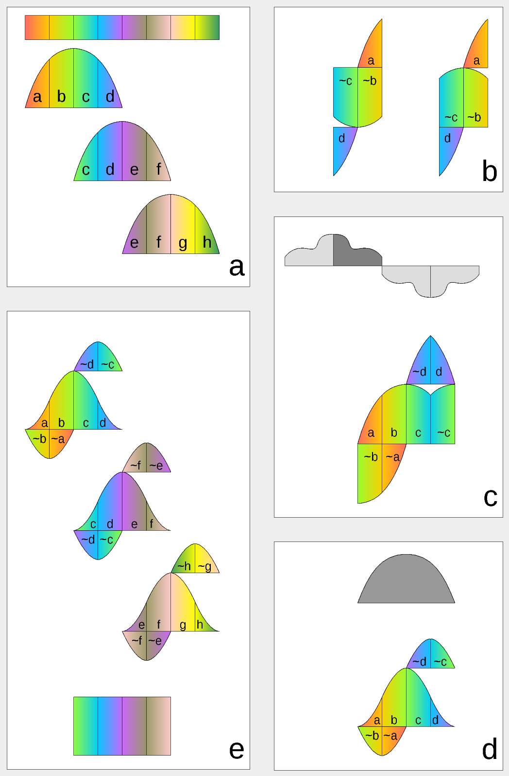
Figure 1. Complex Lapped Transform with DCT-IV/DST-IV: time-domain aliasing cancellation (TDAC) property. a) selection of overlapping input subsequences 2*N-long, multiplication by sine window; b) creating N-long sequences for DCT-IV (left) and DST-IV (right); c) (after frequency domain processing) extending N-long sequence using DCT-IV boundary conditions (DST-IV processing is similar); d) second multiplication by sine window; e) combining partial data
There is another issue related to the space-variant kernels. Fractional pixel shifts are required for multiple steps of the processing: aberration correction (obvious in the case of the lateral chromatic aberration), image rectification before matching that accounts for lens optical distortion, camera orientation mismatch and epipolar geometry transformations. Traditionally it is handled by the image rectification that involves re-sampling of the pixel values for a new grid using some type of the interpolation. This process distorts the signal data and introduces non-linear errors that reduce accuracy of the correlation, that is important for subpixel disparity measurements. Our approach completely eliminates resampling and combines integer pixel shift in the pixel domain and delegates the residual fractional pixel shift (±0.5 pix) to the FD, where it is implemented as a cosine/sine phase rotator. Multiple sources of the required pixel shift are combined for each tile, and then a single phase rotation is performed as a last step of pixel domain to FD conversion.
Frequency Domain Conversion with the Modulated Complex Lapped TransformModulated Complex Lapped Transform (MCLT)[3] can be used to split input sequence into overlapping fractions, processed separately and then recombined without block artifacts. Popular application is the signal compression where “processed separately” means compressed by the encoder (may be lossy) and then reconstructed by the decoder. MCLT is similar to the MDCT that is implemented with DCT-IV, but it additionally preserves and allows frequency domain modification of the signal phase. This feature is required for our application (fractional pixel shifts and asymmetrical lens aberrations modify phase), and MCLT includes both MDCT and MDST (that use DCT-IV and DST-IV respectively). For the image processing (2d conversion) four sub-transforms are needed:
- horizontal DCT-IV followed by vertical DCT-IV
- horizontal DST-IV followed by vertical DCT-IV
- horizontal DCT-IV followed by vertical DST-IV
- horizontal DST-IV followed by vertical DST-IV
Figure 1 illustrates the principle of TDAC (time-domain aliasing cancellation) that restores initial data from the series of individually converted subsections after seemingly lossy transformations. Step a) shows the 2*N long (in our case N=8) data subsets extraction, each subset is multiplied by a window function. It is a half period of the sine function, but other windows are possible as long as they satisfy the Princen-Bradley condition. Each of the sections (a…h) corresponds to N/2 of the input samples, color gradients indicate input order. Figure 2b has seemingly lossy result of MDCT (left) and MDST (right) performed on the 2*N long input (a,b,c,d) resulting in N-long (– c ~ –d,a– b ~ ) – tilde indicates time-reversal of the subsequence (image has the gradient direction reversed too). Upside-down pieces indicate subtraction, up-right – addition. Each of the 2*N → N transforms is irreversible by itself, TDAC depends on the neighbor sections.
Figure 1c shows the first step of original sequence restoration, it extends N-long sequence using DCT-IV boundary conditions – it continues symmetrically around left boundary, and anti-symmetrically around the right one (both around half-sample from the first/last one), behaving like a first quadrant (0 to π/2) of the cosine function. Conversions for DST branch are not shown, they are similar, just extended like a first quadrant of the sine function.
The result sequence of step c) (now 2*N long again) is multiplied by the window function for the second time in step d), the two added terms of the last column (d and c~) are swapped for clarity.
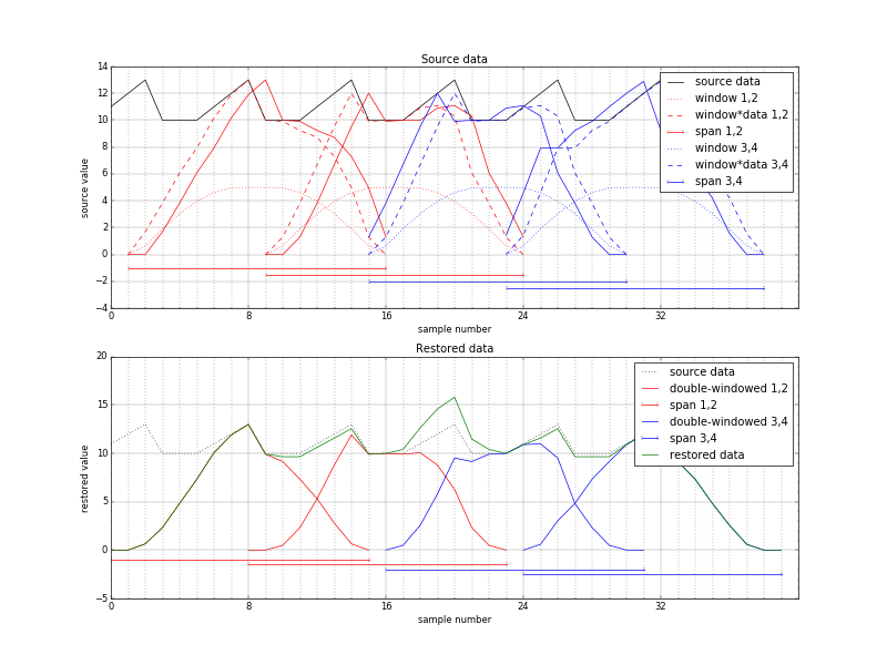
Figure 2. Space-variant phase shift (extra overlap), source-centered window. Distorted reconstruction in the center
The last image e) places result of the step d) and those of similarly processed subsequences (c,d,e,f) and (e,f,g,h) to the same time line. Fraction (d~ ,c~ ) of the first block compensates (–d~ ,– c~ ) of the second, and (f~,e~ ) of the second – (–f~,–e~ ) of the third. As the window satisfies Princen-Bradley condition, and it is applied twice, the c columns of the first and second block when added result in c segment of the original sequence. The same is true for the d, e, and f columns. First and last N samples are not restored as there are no respective left and right neighbors to be processed.
Space-variant shift and TDAC propertyModified discrete cosine and sine transforms exhibit a perfect reconstruction property when input sequence is split into regular overlapping intervals and this is the case for many applications, such as audio and video compression. But what happens in the case of a space-variant shift? As the total shift is split into integer and symmetrical fractional part even smooth variation of the required shift for the neighbor sample sequences there will be places where the required shift crosses ±0.5 pix boundaries. This will cause the overlap to be N±1 instead of exactly N and the remaining fractional pixel shift will jump from +0.5 pix to -0.5pix or vice versa.
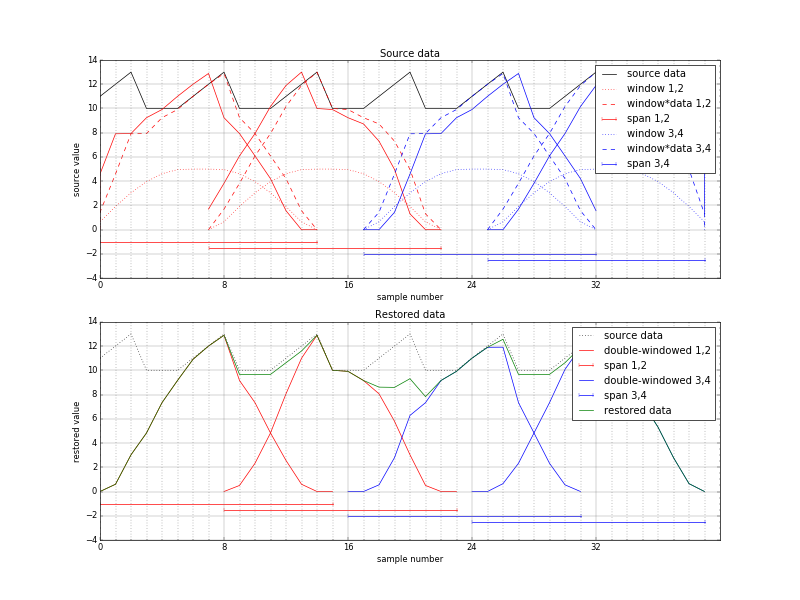
Figure 3. Space-variant phase shift (reduced overlap), source-centered window. Distorted reconstruction in the center
Such condition is illustrated in Figure 2, where fractional pixel shift is increased to ±1.0 instead of ±0.5 to avoid signal shape distortion caused by a fractional shift. The sine window is also modified accordingly to have zeros on both ends and so to have a flat top, but it still satisfies Princen-Bradley condition. The sawtooth waveform represents input signal that has large pedestal = 10 and a full amplitude of 3. The two left input intervals (1 to 16 and 9 to 24) are shown in red, the two right ones (15 to 30 and 23 to 38) are blue. These intervals have extra overlap (N+2) between red and blue ones. Dotted waveforms show window functions centered around input intervals, dashed – inputs multiplied by the windows. Solid lines on the top plot show result of the FD rotation resulting in 1 shift to the right for the red subsequences, to the left – by the blue ones.
The bottom plot of Figure 2 is for the “rectified image”, where the overlapping intervals are spread evenly (0-15, 8-23, 16-31, 24-39), the restored data is multiplied by the windows again (red and blue solid lines) and then added together (dark green waveform) in an attempt to restore the original sawtooth.
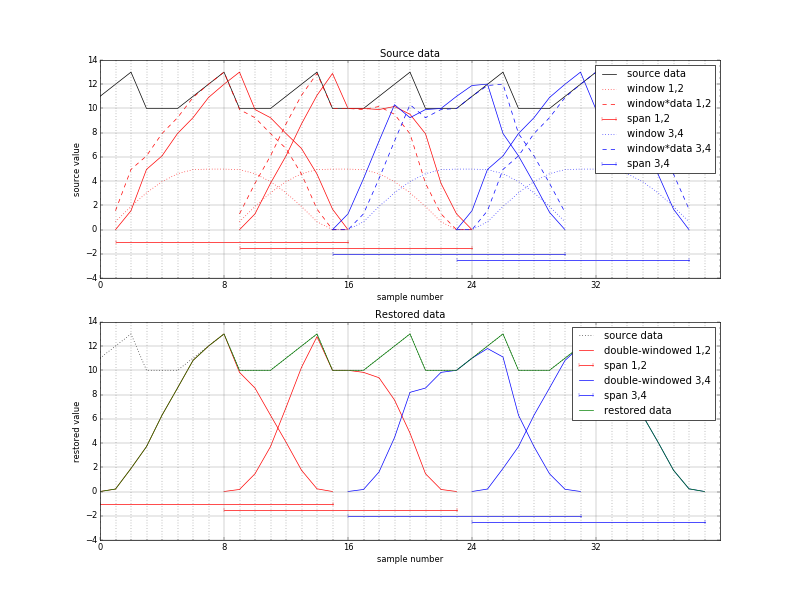
Figure 4. Space-variant phase shift (extra overlap), modified window. Correct reconstruction
There is an obvious problem in the center where the peak is twice higher than the center sawtooth (dotted waveform). It is actually a “wrinkle” caused by the input signal pedestal that was pushed to the center by the increased overlap of the input, not by the sawtooth shape. The FD phase shift moved windowed input signal, not just the input signal. So even if the input signal was constant, left two windows would be shifted right by 1, and right ones – left by one sample, distorting their sum. Figure 3 illustrates the opposite case where the input subsequences have reduced rather than increased overlap and FD phase rotation moves windowed data away from the center – the restored signal has a dip in the middle.
This problem can be corrected if the first window function used for input signal multiplication takes the FD shift into account, so that the input windows after phase rotation match the output ones. Signals similar to those in Figure 2, but with appropriately offset input windows (dotted waveforms are by 1 pixel asymmetrical) are presented in Figure 4. It shows perfect reconstruction (dark green line) of the offset input sawtooth signal.
Figure 5. Space-variant phase shift (reduced overlap), modified window. Correct reconstruction[/caption] Figure ? illustrates the correct reconstruction of the input data of Figure 3 made with the input window function modified to match the FD phase rotation. --> Implementation of the MCLT for the Monochrome 16×16 Pixel Tiles
Figure 5. MCLT converter for the 16×16 pixel tiles
The MCLT converter illustrated in Figure 5 takes an array of 256 pixel samples and processes them at the rate of 1 pixel per clock, resulting in 4 of the 64 (8×8) arrays representing FD transformation of this tile. Converter incorporates phase rotator that is equivalent to the fractional pixel shifter with 1/128 pixel resolution. Multiple pixel tiles tiles can be processed immediately after each other or with a minimal gap of 16 pixels needed to restore the pipeline state. Fold sequencer receives start signal and simultaneously two 7-bit fractional pixel X and Y shifts in 1/128 increments (-64 to +63). Pixel data is received from the read-only port of the dual-port memory (input tile buffer) filled from the external DDR memory. Fold sequencer generates buffer addresses (including memory page number) and can be configured for various buffer latency.
Figure 6. DCT-IV and DST-IV basis functions for N=8
Fold sequencer simultaneously generates X and Y addresses for the 2-port window ROM that generates window function (it is a half-sine as discussed above) values that are combined by a multiplier as the 2-d window function is separable. Each of the dimensions calculate window values with appropriate subpixel shift to allow space-variant FD processing. Mapping from the 16×16 to 8×8 tiles is performed according to Figure 1b for each direction, resulting in four 8×8 tiles for DCT/DCT (horizontal/vertical), DST/DCT, DCT/DST and DST/DST future processing, Each of the source pixels contribute to all 4 of the 8×8 arrays, and each corresponding elements of the 4 output arrays share the same 4 contributing pixels – just with different signs. That allows to iterate through the source pixels in groups of 4 once, multiply them by appropriate window values and in 4 cycles add/subtract them in 4 accumulators. These values are registered and multiplexed during the next 4 cycles feeding 512×25 DTT input buffer (DTT stands for Discrete Trigonometric Transform – a collective name for both DCT and DST).
“Folded” data stored in the 512×25 DTT input buffer is fed to the 2-dimensional 8×8 pixel DTT module. It is similar to the one described in the DCT-IV implementation blog post, it was just modified to allow all 4 DTT variants, not just the DCT/DCT described there. This was done using the property of DCT-IV/DST-IV that DST-IV can be calculated as DCT-IV if the input sequence is reversed (x0 ↔ x7, x1 ↔ x6, x2 ↔ x5, x3 ↔ x4) and sign of the odd output samples (y1, y3, y5, y7) is inverted. This property can be seen by comparing plots of the basis functions in Figure 6, the proof will be later in the text.
Figure 7. Frequency domain phase rotator
Another memory buffer is needed after the 2d DTT module as it processes one of four 64-pixel transforms at a time, and the phase rotator (Figure 7) needs simultaneous access to all 4 components of the same FD sample. These 4 components are shown on the left of the diagram, they are multiplied by 4 sine/cosine values (shown as CH, SH, CV and SV) and then combined by the adders/subtracters. Total number of multiplications is 16, and they have to be performed it 4 clock cycles to maintain the same data rate through all the MCLT converter, so 4 multiplier-accumulator modules are needed. One FD point calculation uses 4 different sine/cosine coefficients, so a single ROM is sufficient. The phase rotator uses horizontal and vertical fractional pixel shift values for the second time (first was for the window function) and combines them with the multiplexed horizontal and vertical indexes (3 bits each) as address inputs of the coefficient ROM. Rotator provides rotated coefficients that correspond to the MCLT transform of the pixel data shifted in both horizontal and vertical directions by up to ±0.5 pix at a rate of 1 coefficient per clock cycle, providing both output data and address to the external multi-page memory buffer.
Modulated Complex Lapped Transform for the Bayer Mosaic Color Images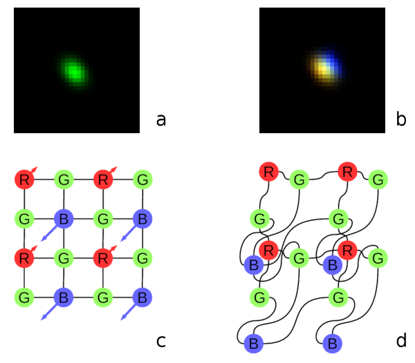
Fig. 8. Lateral chromatic aberration and the Bayer mosaic: a) monochrome (green) PSF, b) composite color PSF, c) Bayer mosaic of the sensor (direction of aberration shown), d) distorted mosaic matching chromatic aberration of b).
Most camera applications use color image sensors that provide Bayer mosaic color data: one red, one blue and two diagonal green pixels in each 2×2 pixel group. In old times image senor pixel density was below the lenses optical resolution and all the cameras performed color interpolation (usually bilinear) of the “missing” colors. This process implied that each red pixel, for example, had four green neighbors (up, down, left and right) at equal distance, and 4 blue pixels located diagonally. With the modern high-resolution sensors it is not the case, possible distortions are shown on Figure 8 (copied from the earlier post). More elaborate “de-mosaic” processing involves non-linear operations that would influence sub-pixel correlation results.
As the simple de-mosaic procedures can not be applied to the high resolution sensors without degrading the images, we treat each color subchannel individually, merging results after performing the optical aberration correction in the FD, or at least compensating the lateral chromatic aberration that causes pixels x/y shift.
Channel separation means that when converting data to the FD the input data arrays are decimated: for green color only half of the values (located in a checkerboard pattern) are non-zero, and for red and blue subchannels – only quarter of all pixels have non-zero values. The relative phase of the remaining pixels depends on the required integer pixel offset (only ±0.5 are delegated to the FD) and may have 2 values (black vs. white checkerboard cells) for green, and 4 different values (odd/even for each of the horizontal/vertical directions independently) for red and blue. MCLT can be performed on the sparse input arrays the same way as on the complete 16×16 ones, low-pass filters (LPF) may be applied on the later processing stages (LPF may be applied to the deconvolution kernels used for aberration correction during camera calibration). It is convenient to multiply red and blue values by 2 to compensate for the smaller number of participating pixels compared to the green sub-channel.
Direct approach to calculate FD transformation of the color mosaic input image would be to either run the monochrome converter (Figure 5) three times (in 256*3=768 clock cycles) masking out different pixel pattern each time, or implement the same module (including the input pixel buffer) three times to achieve 256 clock cycle operation. And actually the 16×16 pixel buffer used in monochrome converter is not sufficient – even the small lateral chromatic aberration leads to mismatch of the 16×16 tiles for different colors. That would require using larger – 18×18 (for minimal aberration) pixel buffer or larger if that aberration may exceed a full pixel.
Luckily MCLT that consists of MDCT and MDST, they it turn use DCT-IV and DST-IV that have a very convenient property when processing the Bayer mosaic data. Almost the same implementation as used for the monochrome converter can transform color data at the same 256 clock cycles. The only part that requires more resources is the final phase rotator – it has to output 3*4*64 values in 256 clock cycles so three instances of the same rotator are required to provide the full load of the rest of the circuitry. This almost (not including rotators) triple reduction of the MCLT calculation resources is based on “folding” of the input data for the DTT inputs and the following DCT-IV/DST-IV relation.
Relation between DCT-IV and DST-IVDST-IV is equivalent to DCT-IV of the input sequence, where all odd input samples are multiplied by -1, and the result values are read in the reversed order. In the matrix form it is shown in (1) below:
.equation td{text-align:center; vertical-align:middle; } td.eq-no{ width:5%; } table.equation { width:100%; } DST IV = [ 0 1 1 1 ⋅⋅⋅ 1 0 ] ⋅ DCT IV ⋅ [ 1 0 -1 1 ⋅⋅⋅ 0 -1 ] (1)Equations (2) and (3) show definitions of DCT-IV and DST-IV[4]:
DCT IV (k) = 2N ⋅ ∑ l=0 N–1 cos( π N ⋅(l+12) ⋅(k+12) ) (2) DST IV (k) = 2N ⋅ ∑ l=0 N–1 sin( π N ⋅(l+12) ⋅(k+12) ) (3)The modified by (1) DST-IV can be re-writted as the two separate sums for even (l=2*m) and odd (l=2*m+1) input samples and by replacing output samples k with reversed (N-1-k). Then after removing full periods (n*2*π) and applying trigonometric identities it can be converted to the same value as DST-IV:
DCT mod IV (k) = 2N ⋅ ( ∑ m=0 N/2–1 cos( π N ⋅(2⋅m+12) ⋅((N–1–k)+12) ) – ∑ m=0 N/2–1 cos( π N ⋅(2⋅m+32) ⋅((N–1–k)+12) ) ) = 2N ⋅ ( ∑ m=0 N/2–1 cos( π N ⋅( 12⋅N – (2⋅m+12) ⋅(k+12) ) ) – ∑ m=0 N/2–1 cos( π N ⋅( 32⋅N – (2⋅m+32) ⋅(k+12) ) ) ) = 2N ⋅ ( ∑ m=0 N/2–1 cos( –π2 +π N ⋅(2⋅m+12) ⋅(k+12) ) – ∑ m=0 N/2–1 cos( π2 + π N ⋅(2⋅m+32) ⋅(k+12) ) ) = 2N ⋅ ( ∑ m=0 N/2–1 sin( π N ⋅(2⋅m+12) ⋅(k+12) ) + ∑ m=0 N/2–1 sin( π N ⋅(2⋅m+32) ⋅(k+12) ) ) = DST IV (k) (4) Two-dimensional MCLT Symmetries for the Bayer Mosaic Sub-arraysAs shown in Figure 1b, the 2*N-long input sequence of four fragments (a,b,c,d) is folded in N-long sequence (5) for DCT-IV input:
(a,b,c,d) ⟶ (– c ~ –d,a– b ~ ) (5)and (6) – for DST-IV:
(a,b,c,d) ⟶ ( c ~ –d,a+ b ~ ) (6)where tilde “~” over the name indicates reversal of the segment. Such direction reversal for the sequences of even length (N/2=4 in our case) swaps odd- and even-numbered samples. Each of the halves of each of (5) and (6) show that both have the same (–d,a) for direct and differ in sign for reversed: (– c~ , –b~ ) and ( c~ , b~ ) terms. Each of the input samples appears exactly once in each of the DCT-IV and DST inputs. Even samples of the input sequence contribute identically to the even samples of both output sequences (through a an d) and contribute with the opposite signs to the odd output samples (through b and c). And similarly the odd-numbered input samples contribute identically to the odd-numbered output samples and with the opposite sign to the even ones.
So, sparse input sequence with only non-zero values at even positions result in both DCT-IV and DST-IV having the same values at even positions and multiplied by -1 – in the odd. Odd-only input sequences result in same values in odd positions and negatives – in the even ones.
Now this property can be combined to the previously discussed DST-IV to DCT-IV relation and extended to the two-dimensional Bayer mosaic case. We can start with the red and blue channels that have 1-in-4 non-zero pixels. If the non-zero pixels are in the even columns, then after first horizontal pass the DST-IV output will differ from the DCT-IV only by the output samples order according to (1), as even input values are the same, and odd are negated. Reversed output coefficients order for the horizontal pass means that the DST-IV will be just horizontally flipped with respect to the DCT-IV one. If the non-zero input was for the odd columns, then the DST-IV output will be reversed and negated compared to the DCT-IV one.
The second (vertical) pass is applied similarly. If original pattern had non-zero even rows, the result of vertical DST-IV would be the same as those of the DCT-IV after a vertical flip. If the odd rows were non-zero instead – the result will be vertically flipped and negated with respect of the DCT-IV one.
This result means that for the 1-in-4 Bayer mosaic array only one DCT-IV/DCT-IV transform is need. The three other DTT combinations may be obtained by flipping the DCT-IV/DCT-IV output horizontally and/or vertically and possibly negating all the data. Reversal of the readout order does not require additional hardware resources (just a few gates for a little fancier memory address counter). Data negation is also “free” as it can easily be absorbed by the phase rotator that already has adders/subtracters and just needs an extra inversion sign control. Flips do not depend on the odd/even columns/rows, only negation depends on them.
Green channel has non-zero values in either (0,0) and (1,1) or (0,1) and (1,0) positions. So it can be considered as a sum of two 1-in-4 channels described above. In the (0,0) case neither horizontal, no vertical DST-IV inverts sign, and (1,1) inverts both, so the DST-IV/DST-IV does not have any inversion, and it will stay true for the green color – combination of (0,0) and (1,1). We can not compare DCT-IV/DCT-IV with ether DST-IV/DCT-IV or DCT-IV/DST-IV, but these two will have the same sign compared to each other (zero or double negation). So the DST-IV/DST-IV will be double-flipped (both horizontally and vertically) version of the DCT-IV/DCT-IV output, and DCT-IV/DST-IV – double flipped version of DST-IV/DCT-IV, and calculation for this green pattern requires just two of the 4 DTT operations. Similarly, for the (0,1)/(1,0) green pattern DST-IV/DST-IV will be double-flipped and negated version of the DCT-IV/DCT-IV output, and DCT-IV/DST-IV – double-flipped and negated version of DST-IV/DCT-IV.
Combining results for all three color components: reg, blue and green, we need total of four DTT operations on 8×8 tiles: one for red, one for blue and 2 for green component instead of twelve if each pixel had full RGB value.
Implementation of the MCLT for the Bayer Mosaic Pixel Tiles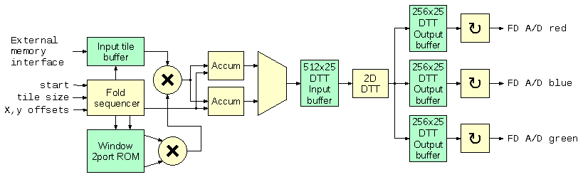
Figure 9. MCLT converter for the Bayer mosaic tiles
MCLT converter for the Bayer Mosaic data shown in Figure 9 is similar to the already described converter for the monochrome data. The first difference is that now the Fold sequencer addresses larger source tiles – it is run-time configurable to be 16×16, 18×18, 20×20 or 22×22 pixels. Each tile may have different size – this functionality can be used to optimize external memory access: use smaller tiles in the center areas of the sensor with lower lateral chromatic aberrations, read larger tiles in the peripheral areas with higher aberrations. The extended tile should accommodate all three color shifted 16×16 blocks as shown in Figure 10.
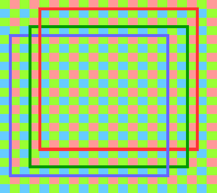
Figure 10. Example color channels 16×16 pixel tiles mismatch due to the chromatic aberration
The start input triggers calculation of all 3 colors, it can appear either each 256-th clock cycle or it needs to wait for at least 16 cycles after the end of the previous tile input if started asynchronously. X/Y offsets are provided individually for each color channel and they are stored in a register file inside the module, the integer top-left corner offset is provided separately for each color to simplify internal calculations.
Dual-port window ROM is the same as in the monochrome module, both horizontal and vertical window components are combined by a multiplier and then the result is multiplied by the pixel data received from the external memory buffer with configurable latency.
There are only two (instead the four for monochrome) accumulators required because each of the “folded” elements of the 8×8 DTT inputs has two contributor source pixels at most (for green color), while red and blue use just a single accumulator. Red color is processed first, then blue, and finally green. For the first ones only the DCT-IV/DCT-IV input data is prepared (in 64 clock cycles each), green color requires DST-IV/DCT-IV block additionally (128 clock cycles).
DTT output data goes to three parallel dual-port memory buffers. Red and blue channels each require just single 64-element array that later provides 4 different values in 4 clock cycles for horizontally and vertically flipped data. Green channel requires 2*64 element array. These buffers are filled one at a time (red, blue, green) and each of them feed corresponding phase rotator. Rotator outputs need 256 cycles to provide 4*64=256 FD values, the symmetry exploited during DTT conversion is lost at this stage. The three phase rotators can provide output addresses/data asynchronously or the green and blue outputs can be delayed and output simultaneously with the green channel, sharing the external memory addresses.
MCLT Converter for the Bayer Mosaic Tiles Simulation and Comparison to the Software Post-processing results
Figure 11. MCLT converter for the Bayer mosaic simulation
Results of the simulation of the MCLT converter are shown in Figure 11. Simulation ran with the clock frequency set to 100 MHz, the synthesized code should be able to run at at least 250 MHz in the Zynq SoC of the NC393 camera – at the same rate as is currently used for the data compression – all the memories and DSPs are fully buffered. Simulation show processing of the 3 tiles: two consecutive and the third one after a minimal pause. The data input was provided by the Java code that was written for the post-processing of the camera images, the same code generated intermediate results and the output of the MCLT conversion. Java used code involved double precision floating point calculations, while the RTL code is based on fixed-point calculations with the precision of the architecture DSP primitives, so there is no bit-to-bit match of the data, instead there is a difference that corresponds to the width of the used data words.
ResultsThe RTL code (licensed under GNU GPLv3+) developed for the MCLT-based frequency domain conversion of the Bayer color mosaic images uses almost the same resources as the monochrome image transformation for the tiles of the same size – three times less than a full RGB image would require. Input window function modification that accounts for the two-dimensional fractional pixel shift and the post-transform phase rotators allow to avoid re-sampling for the image rectification that degrades sub-pixel resolution.
This module is simulated with Icarus Verilog (a free software simulator), results are compared to those of the software post-processing used for the 3-d scene reconstruction of multiple image sets, described in the “Long range multi-view stereo camera with 4 sensors” post.
The MCLT module for the Bayer color mosaic images is not yet tested in the FPGA of the camera – it needs more companion code to implement a full processing chain that will generate disparity space images (DSI) required for the real-time 3d scene reconstruction and/or output of the aberration-corrected image textures. But it constitutes a critical part of the Tile Processor project and brings the overall system completion closer.
References[1] Thiébaut, Éric, et al. “Spatially variant PSF modeling and image deblurring.” SPIE Astronomical Telescopes+ Instrumentation. International Society for Optics and Photonics, 2016. pdf
[2] Řeřábek, M., and P. Pata. “The space variant PSF for deconvolution of wide-field astronomical images.” SPIE Astronomical Telescopes+ Instrumentation. International Society for Optics and Photonics, 2008.pdf
[3] Malvar, Henrique. “A modulated complex lapped transform and its applications to audio processing.” Acoustics, Speech, and Signal Processing, 1999. Proceedings., 1999 IEEE International Conference on. Vol. 3. IEEE, 1999.pdf
[4] Britanak, Vladimir, Patrick C. Yip, and Kamisetty Ramamohan Rao. Discrete cosine and sine transforms: general properties, fast algorithms and integer approximations. Academic Press, 2010.
Updated Poky to Rocko
We have updated the Yocto build system to Poky Rocko released back in October. Here’s a short summary table of the updates:
before after Poky 2.0 (Jethro) 2.4 (Rocko) gcc 5.3.0 7.2.0 linux kernel 4.0 4.9Other packages got updates as well:
- apache2-2.4.18 => apache2-2.4.29
- php-5.6.16 => php-5.6.31
- udev-182 changed to eudev-3.2.2, etc.
This new version is in the rocko branch for now but will be merged into master after some transition period (and the current master will be moved to jethro branch). Below are a few tips for future updates.
It was relatively simple to update the recipes and build the images. Most of the packages were updated to newer versions. One noticeable change is tmp/sysroots/ is not a common location anymore – instead there is the recipe-sysroot/ directory in each recipe’s build directory. Also, our headers didn’t get to the sysroots which got fixed by having:
sysroot_stage_all_append() {
sysroot_stage_dir ${WORKDIR}/headers/include ${SYSROOT_DESTDIR}/usr/include-uapi
}
We had this task in Jethro but there was another variable used ${STAGING_DIR_TARGET} (instead of ${SYSROOT_DESTDIR})
It took most of the time to update it.
Luckily our drivers didn’t break but there were a few problems:
First, we merged our drivers and patches to make the kernel get built at least. After building the kernel the serial output didn’t work – the fix was to switch to earlycon in bootargs in the device tree (in 4.0 ealyprintk still worked):
before:
chosen {
bootargs = "cma=128M console=ttyPS0,115200 root=/dev/mmcblk0p2 rw earlyprintk rootwait rootfstype=ext4";
linux,stdout-path = "/amba@0/serial@e0000000";
};
after:
chosen {
bootargs = "earlycon cma=128M root=/dev/mmcblk0p2 rw rootwait rootfstype=ext4";
stdout-path = "serial0:115200n8";
};
Next, there was no ethernet. After some time of debugging the problem was with the device tree again:
before:
phy3: phy@3 {
compatible = "atheros,8035";
device_type = "ethernet-phy";
reg = <0x3>;
};
after:
phy3: phy@3 {
/* Atheros 8035 */
compatible = "ethernet-phy-id004d.d072";
/* compatible = "ethernet-phy-ieee802.3-c22";*/
device_type = "ethernet-phy";
reg = <0x3>;
};
The compatible field has to be in a certain format. See the docs.
The next thing has Xilinx switched from xlnx,ps7-ethernet-1.00.a to cdns,zynq-gem (see arch/arm/boot/dts/zynq-7000.dtsi). Didn’t track when – both drivers work. The cdns,zynq-gem is in the mainline, the other is not.
And the last change to the ethernet driver was adding the fixup for Atheros 8035, the network chip we use.
Then the bitstream wouldn’t get programmed. It was Xilinx’s problem – new gcc was opting away some of the variables (dma_done) in the driver – they fixed the kernel but didn’t change the hash of the linux-xlnx in the recipe yet (linux-xlnx_2017.3.bb). So, it’s probably coming to 2017.4.
Xilinx has changed some of its default config variables and in 4.9 there are a few new dependencies here and there.
The changes made to our config (elphel393.cfg) which is added to the default config for zynq devices:
# This option is for FPGA part
CONFIG_XILINX_DEVCFG=y
# prints time before messages
CONFIG_PRINTK_TIME=y
# dependency for DYNAMIC_DEBUG=y
CONFIG_DEBUG_FS=y
# turned off because old:
CONFIG_XILINX_PS_EMAC=n
CONFIG_XILINX_EMACLITE=n
CONFIG_XILINX_AXI_EMAC=n
udev package switched from udev-182 changed to eudev-3.2.2. udev-182 can copy static device files from /lib/udev/devices/, eudev-3.2.2 does not do this – created a new rule:
ACTION=="add", RUN+="/usr/bin/rsync -a /lib/udev/devices/ /dev/"
This rule adds up ~6 secs to boot time for some reason vs almost nothing if run from the camera init script init_elphel393.py
- Reminder: the system boots into initramfs first and runs init built by initramfs-live-boot. The script runs switch_root in the end. udev daemon gets killed and restarted
Assembling Long Range Stereo Camera
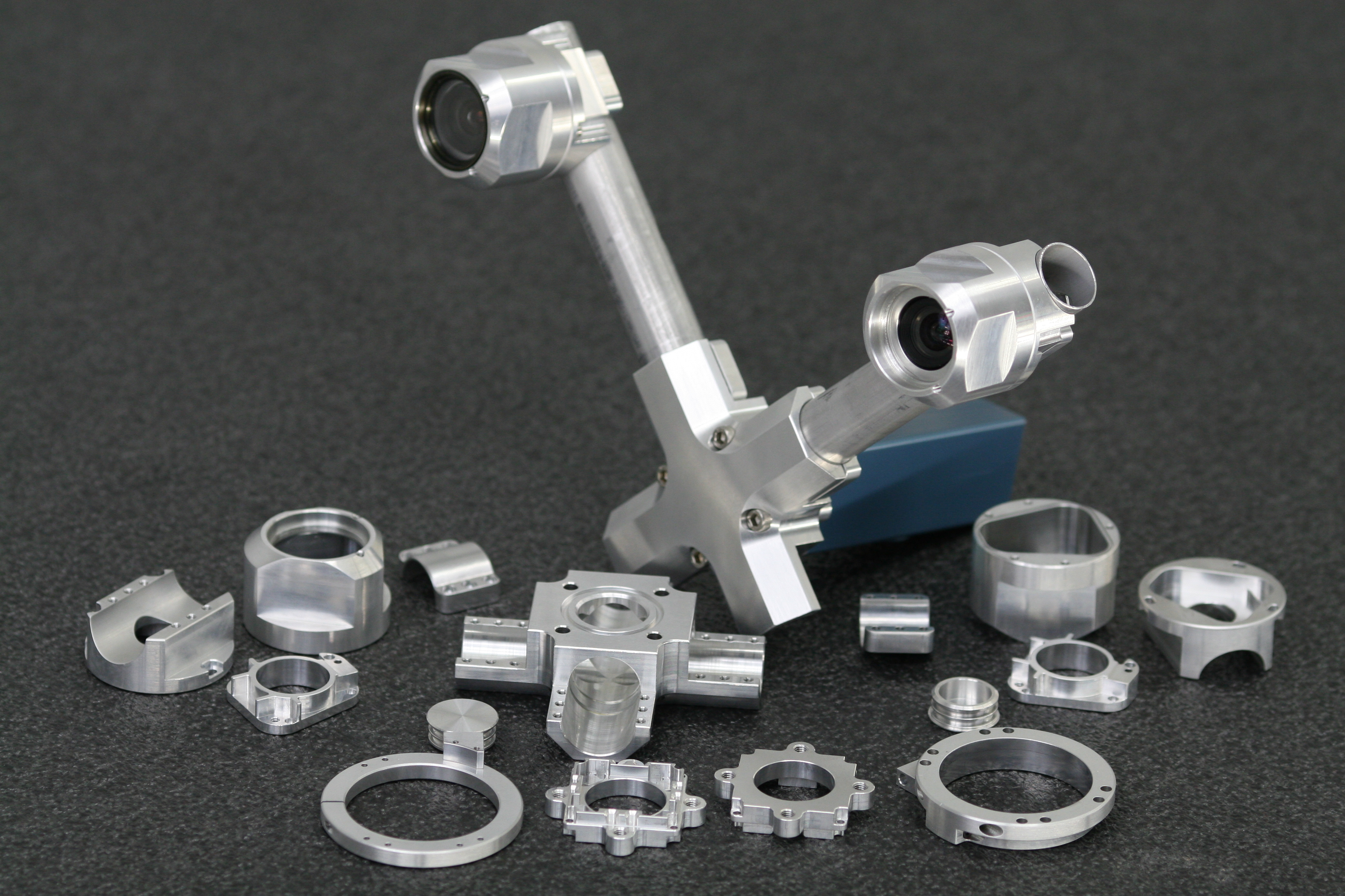
MNC393-XCAM partial assembly and parts
The long anticipated parts for the Long range camera have arrived!
The mechanical parts for the MNC393-XCAM – Long Range Multi-view Stereo Camera are machined, tested, and ready to be anodized. This enables us to have the X-camera assembled before the winter holidays. The holiday break will provide a good opportunity to test the camera, capture new photos, and create robust 3D models from calibrated images.
The titanium X-frame of the camera ensures thermal stability required for continuous accuracy of 3D measurements. The aluminum enclosure and sealed lens filters weatherproof the system allowing for the proposed outdoor use of the camera.
We intend to assemble two cameras: one with a 150 mm distance between the sensors and another with a longer baseline. The expected accuracy for the camera with the shorter baseline is greater than 10% at a 200 meter distance. We have achieved 10% accuracy with H-camera with calibrated sensors, even though the 3D-printed parts were not thermally stable and some error was accumulated over time. It was a very pleasant surprise that the software was still able to deal with somewhat un-calibrated images and detect distances very accurately, creating impressive 3D-scenes: Scene_viewer The second camera will have a 280 mm distance between sensors, which is determined by the longest FPC cables we can use without signal losses. It promises to double the measured distance with the same degree of accuracy, therefore an extremely long range 3D-scenes will be produced.
The Long Range Multi-View Stereo Camera with 4 sensors MNC393-XCAM is planned for release in early 2018.
Drupal, WordPress, Mediawiki, Mail Archive, Gitlab – all in one web site
Multiple Subdomains for the Same Web Site
It is a common case when a company or organization uses multiple content management systems (CMS) and specialized web application to organize its web presence. We describe here how Elphel handles such CMS variety and provide the source code that can be customized for other similar sites.
We currently use the following CMS and web applications:
- Drupal as a general purpose CMS for the main site
- WordPress for the development blogs
- Mediawiki for the wiki-based documentation.
- Mailman (self hosted) and Mail Archive (external site) for the mailing list that is our main channel of the user technical support
- Gitlab CE for the code and other version-controlled content. We used Github but switched to self-hosted Gitlab CE following FSF recommendations
- Other customized versions of FLOSS web applications, such as OSTicket for support tickets and FrontAccounting for inventory and production
- In-house developed free software web applications, such as x3dom-based 3D scene and map viewer, 3D mechanical assembly viewer available for the assemblies and mechanical components on the wiki, WebGL Panorama Viewer/Editor.
Figure 1. Elphel web site on a desktop screen
When users visit company web site they expect to have well organized and logically solid navigation to get the information they came for. There are multiple ways how to combine several applications – for example, it is possible to add wiki to WordPress or use it with Gitlab repositories. Of course it is theoretically possible to develop a web site where all the information in available in these applications will be properly cross-linked and stay current. It may also be possible to customize one of the CMS to handle all the needs, but that would require significant web development resources. For a small company following that path the required number of web developers may easily exceed the number of hardware, FPGA and software developers.
On the other hand the small company size should not be an excuse – why the web site visitors can not find the information they are looking for. For us it was a very clear signal when our long time users asked if we can email them mechanical drawings of the camera boards and components. For us that meant a bad web site usability – for years we have this information for some 900+ standard and machined parts available in our wiki: DXF and PDF for 2-d drawings, STEP files for 3d in our wiki: 393 series and previous 353 series. Camera mechanical assemblies can be navigated with the x3dom-based viewer.
Improving Navigation of the Composite Web SiteAs we were not going to give up simultaneous use of multiple content management systems (we needed functionality of each of them) we were looking for the following improvements of information accessibility:
- to have a common search over all subdomains always available (looking glass icon in the top right corner)
- as we can not cross-link properly all the information, then at least we have to communicate the idea that there are multiple subdomains to our visitors.
Figure 2. Site search for ‘ERS’ (acronym for Electronic Rolling Shutter)
We did try to launch simultaneous search over the main (Drupal) site, wiki, blog (WordPress) and Mail Archive using site-specific requests, but that was available only on the main site, and for Mail Archive we could not add it as it is hosted on the external site. An obvious solution to have site-wide search always accessible, including external sites was to use iframe elements. Figure 2 shows results of simultaneous search for “ERS”, each linking to the corresponding subdomain tab.
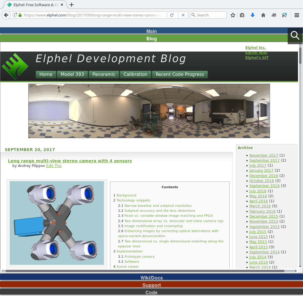
Figure 3. Elphel web site on a small screen
Immitating Multiple Application WindowsAs we have to use iframe elements for multi-site search we can use the framed layout to tell visitors that instead of a single web site with a consistent navigation there are in fact multiple subdomains, each having different structure and navigation. Instead of a single browser window or tab we are presenting the web site as a stack of individual windows on a desktop as shown on Figure 1. Most web sites do not use full width of the modern computer desktop and have useful content width of just 800-1100 pixels – that gives some room to show parts of the subdomain pages that are out of focus in our case. For the not as wide screens (or browser windows) such as on mobile devices, the page layout is different (Figure 3) – subdomains that are currently out of focus are shown as colored horizontal bars. Navigation is rather intuitive – mouse click on the background tab brings it to focus, following links that lead to the other subdomain (e.g. from the blog tab to wiki) brings the corresponding page to focus and shows linked page there, avoiding the case when there will be two wiki tabs and no blog ones. External links open in new browser tabs – that also helps to keep multi-site structure intact.
Each subdomain page title (Main, Blog, Wiki/Docs…) is a link to the content shown in the current iframe element. Following that link or using “Copy Link Location” from a context menu opens just that subdomain page alone or copies its address to use it as a bookmark or send over email or post in social media.
Redirection and Canonical URLsNext step after selecting the overall page layout was to decide – how should we show the framed version to the visitors and what URLs to have as canonical for different pages? At that point we had multiple subdomains: https://www3.elphel.com for the main site (Drupal), https://wiki.elphel.com for the wiki (Mediawiki), https://blog.elphel.com for the blogs (WordPress). The default https://www.elphel.com domain was reserved for the top page to open individual subdomains in the iframe elements.
One way to deal with it was to permanently redirect https://www3.elphel.com/* to https://www.elphel.com/www3/*, https://wiki.elphel.com/* to https://www.elphel.com/wiki/*, and so on, and then to rely on https://www.elphel.com/index.php to process the request and open subdomains in respective iframe elements. That would always load all the stack of the pages and may be both intrusive and annoying – visitors may be already aware of the structure of the web site and want just the specific blog post or wiki page. And as iframes are routinely used for serving ads, their functionality may be disabled in the browser of a visitor.
We use the original URLs as canonical (e.g. https://wiki.elphel.com/*, not https://www.elphel.com/wiki/*), so search engines will return them as the results, and then redirect (with temporary 302) requests depending on the referrer. If referrer (HTTP_REFERER) is provided in the request and it does not belong to Elphel domain – open the framed version with focus on the tab with the requested URL. Otherwise, with no referrer (directly entered, received via email, disabled for privacy reasons) or when opening the link from other Elphel page (such as already framed version) the page is opened alone.
Below is the relevant portion of the Apache 2 .htaccess file for the https://blog.elphel.com (there are also WordPress-specific rules and enforcing SSL access (use of https instead of insecure http protocol). Lines 5..7 are to disable redirection for certain groups of addresses. Line 2 discloses the fact (by adding “Vary: Referer” to the headers) that response depends on the referrer page.
#Tell search engines we do not cloak Header always add Vary: Referer RewriteCond %{REQUEST_FILENAME} !-f RewriteCond "%{HTTP_REFERER}" "!^((.*)elphel\.com(.*)|)$" RewriteCond %{REQUEST_URI} !category.*feed RewriteCond %{REQUEST_URI} !^/[0-9]+\..+\.cpaneldcv$ <span style="color:#999999">RewriteCond %{REQUEST_URI} !^/\.well-known/pki-validation/[A-F0-9]{32}\.txt(?:\ Comodo\ DCV)?$</span> RewriteRule ^(.*)$ https://www.elphel.com/blog%{REQUEST_URI} [L,R=302]Such redirection is obviously impossible for external sites as Mail Archive and we did not use it for https://git.elphel.com – in both cases if visitors followed those links from the search engines results, they would not expect such pages to be parts of the well cross-linked company web site.
ImplementationSource code: iframed
The main frame is a single page with iframe elements. The iframes’ addresses are hard coded in the index.php.
To avoid, where possible, displaying the same content in multiple frames window.postMessage() method is used. Link click events in an iframe are blocked and the link data is passed to the main frame via postMessage for analysis following focusing on an iframe with a matching domain and refreshing the links or opening a new tab for external websites.
The following code was added to each controlled subdomain (see elphel_messenger.js):
<script src="https://www.elphel.com/js/elphel_messenger.js"></script> <script> ElphelMessenger.init(); </script> Usability ans SEOWe are trying to improve usability of the company web site that effectively is a collection of subdomains each running different CMS without major investments into the web design. At the same time we were trying to avoid mistakes in SEO (were we do not have much experience) that would make Elphel invisible for the search engines. Our SEO concerns were caused by the following reasons:
- the top (almost like a “frameset” in older HTML days) page itself has very little content – most is provided in the included iframe elements
- the served content depends on the referrer address – that might be considered as “cloaking.”
Knowing nothing how algorithms are distinguishing between cloaking and legitimate referrer redirects (such as visitors geographical location) we assumed that cloaking shows indexing bots some information that is not served to the human visitors. Our case is different – visitors get either exactly the same information as the bots, or the same one plus additional. We indicated that the served content depends on the referrer URL in the response header (so smart bot can try variable values for “referer”). Testing the new web site for half year did not show any negative effect on the web site visibility in the search engines.
But the main question still remains – did we reach our goal to improve web site usability?
- Were we able to communicate the idea that the site consists of multiple loosely-connected subdomains with different navigation?
- Is the framed site navigation intuitive or annoying?
- Does the combined search over multiple subdomains do its job and does it behave as users expect?
Only our visitors can tell us this, user comments are always welcome. And while we do not have a one-click distribution to use this solution for other similar sites (some customization will be needed) our code is available in the Git repository iframed.