Elphel new camera calibration facility
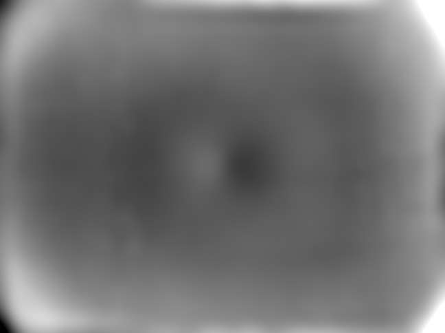
Fig.1. Elphel new calibration pattern
Elphel has moved to a new calibration facility in May 2013. The new office is designed with the calibration room being it’s most important space, expandable when needed to the size of the whole office with the use of wide garage door. Back wall in the new calibration room is covered with the large, 7m x 3m pattern, illuminated with bright fluorescent lights. The length of the room allows to position the calibration machine 7.5 meters away from the pattern. The long space and large pattern will allow to calibrate Eyesis4π positioned far enough from the pattern to be withing depth of field of its lenses focused for infinity, while still keeping wide angular size, preferred for accuracy of measurements.
We already hit the precision limits using the previous, smaller pattern 2.7m x 3.0m. While the software was designed to accommodate for the pattern where each of the nodes had to have individually corrected position (from the flat uniform grid), the process assumed that the 3d coordinates of the nodes do not change between measurements.
The main problem with the old pattern was that the material it was printed on was attached to the wall along the top edge but still had a freedom to slightly move perpendicular to the wall. We noticed that while combining measurements made at different time, as most of our cameras need to be calibrated at several “stations” – positions relative to the target (rotation around 2 axes is performed automatically). We ran calibration during night time to reduce variations caused by vibrations in the building, so next station measurements were performed at different dates. Modified software was able to deal with variations in Z (perpendicular to the surface) direction between station measurements (that actually did help in the overall adjustment of variables), but the shape of the target pattern could change if the temperature in the building was changing during measurements. The PVC material has high thermal expansion, and small expansion in the X,Y directions could cause much higher variations perpendicular when the target is attached to the wall with lower thermal coefficient in multiple points.
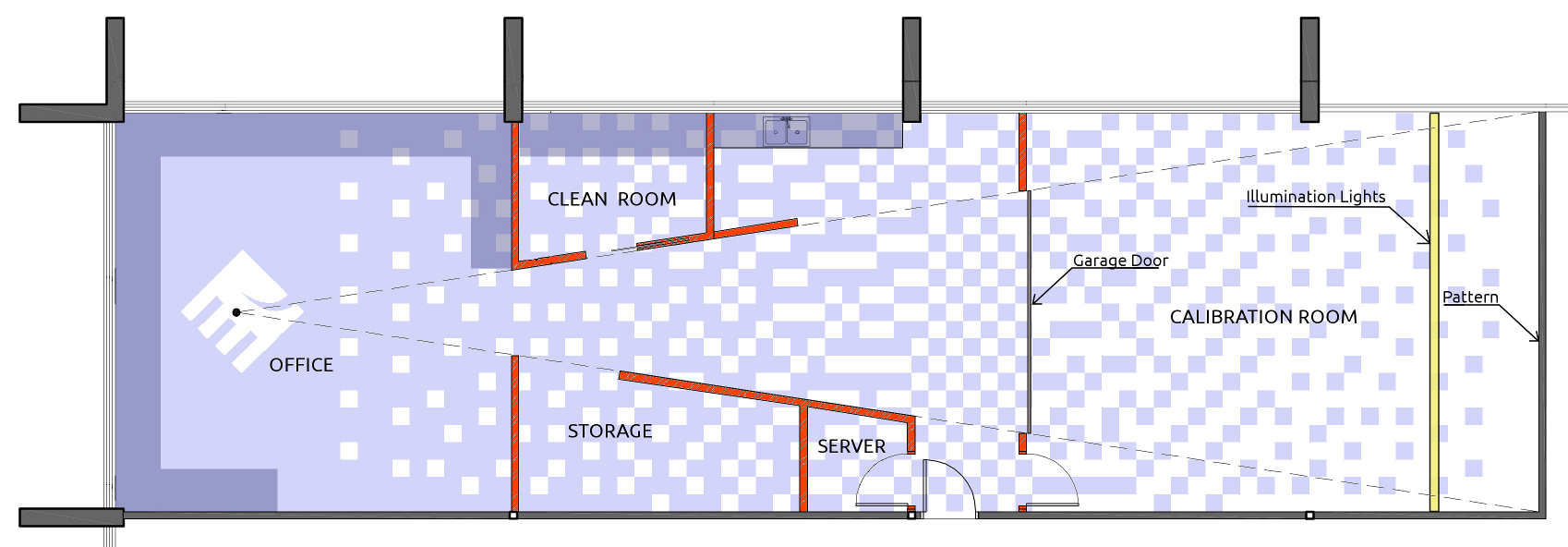
Fig. 2. Floor plan
Calibration RoomThe new space is designed to accommodate various camera calibration procedures.
- First of all we made the pattern as large as possible – it is 7,01m x 3.07m – we even raised the ceiling near the target.
- The target itself is now printed on the film attached to the wall as a wallpaper, so there is no movement relative to the wall, and thermal expansion is defined by a lower coefficient of the drywall. We also provided the air channels inside the wall to make it possible to implement thermal stabilization of the wall.
- The calibration room allows to move camera under test up to 7.5m away from the pattern, the room is separated from the rest of the facility with the wide “garage” door, so changing the lighting conditions outside of the room do not influence calibration.
- Other rooms are designed in such a way that the camera can be moved up to 24 meters from the target (with the garage door open) and have unobstructed view of virtually the full pattern – that may be needed for the long focal length lenses.
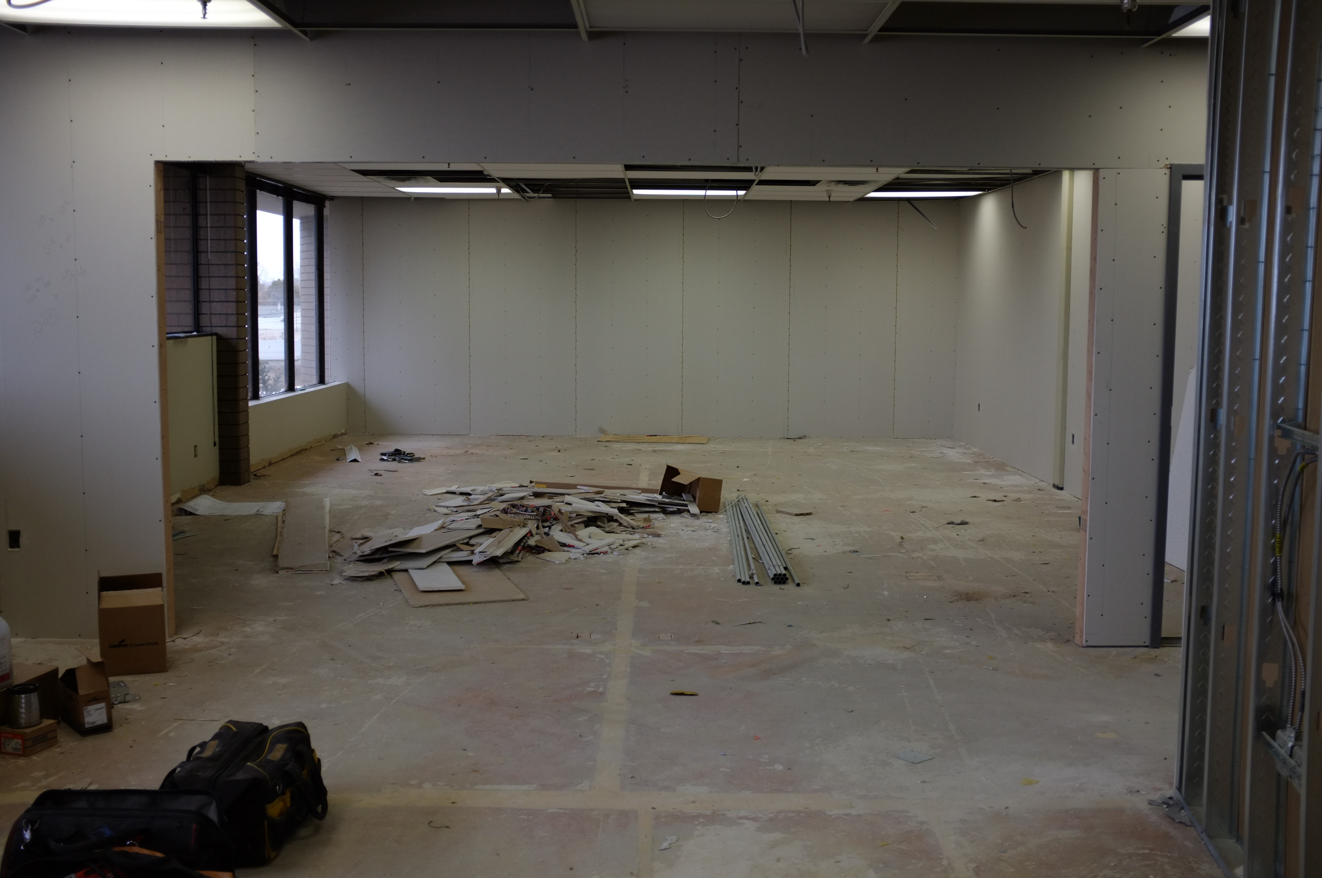
Fig. 3. Pattern wall during construction
Preparing the wall for the target patternDuring construction of the new facility we were carefully watching the progress as our temporary space was located just on the next floor and we were mostly concerned about the quality of the target wall. Yes, software can accommodate for the non-flatness of the wall but it is better to start with the good “hardware” – to achieve subpixel precision the software averages correlation over rather large areas of the image (currently 64×64 pixels) so sharp variations will produce different measurements from different distances or viewing angles. When we first measured the wall flatness, we noticed large steps between the gypsum board panels, so the construction people promised to make it level 5 finish and flatten the surface. They put “mud” all over the wall, sanded it and that removed all of the sharp discontinuities on the target surface, but still leaving some smooth ones up to ±3mm as we measured later with the camera.
When the wall was made flat it had to be prepared for application of the self-adhesive vinyl film, so the wall finish will not make it bubble later. Ideally we wanted it to be able to withstand peeling off the film if we’ll have to do that. When we searched Internet about vinyl film application to the painted wall we found that most fresh paint needs some 60(!) days to cure before the film can be applied. So we decided to go with two-component epoxy paint that requires only one week before the film can be applied. When we inspected that epoxy painted wall (the paint was applied with the regular rollers) – it did not look flat. Well, it was just a roller-painted wall, so it had those small bumps and we were concerned that the vinyl film will conform to these bumps, and if it will – the position “noise” will be higher than what cameras can resolve. So we’ve got more epoxy paint and started a long process of wet-sanding and application of the new paint coats. We have compressed air (used to blow during optical and mechanical assembly) so we thought we’ll just spray the paint instead of rolling it to avoid those bumps that were left even after professional work. Unfortunately, without the needed experience in spray-painting, we adjusted pressure too high, and probably as much as a half of our first coat ended somewhere else, but not on the sprayed wall – the paint droplets were too small. Next coat was better, and in several days we had a wall that seemed to be covered with hard plastic laminate, not just painted.
Installing the patternOur next concern was – how to install the vinyl film? We wanted to have very good match between the individual panels, as it is not possible to have the target printed on a single piece, maximal width of which is just over 1.5m. We hesitated to order professional installation because for regular applications (like vehicle wraps) such sub-millimeter precision is not required. For the really seamless (compared to the precision of the calibration) we needed better than 0.1mm match, but it is possible to just mask out the grid nodes around the seams and disregard them during calibration data processing, so we planned to get to about 0.5mm match.
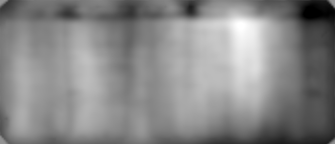
Fig.4. Pattern Z-deviations (perpendicular to the target plane)
Fig. 5. Pattern deviations in X,Y plane
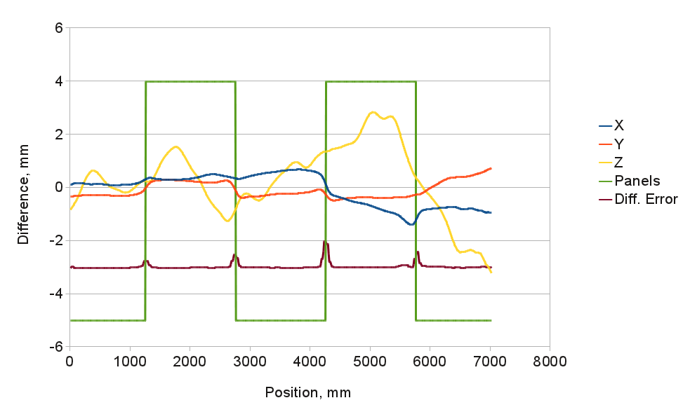
Fig. 6. Pattern deviation from the "ideal" grid (horizontal profile)
We knew people are doing that but still it seemed very difficult to apply 1.5m wide by 3m long “stickers” without wrinkles and bubbles. Web search provided multiple recommendations, but the main thing was to use “wet” method that none of us new before. It involves spraying the wall (and the film on the adhesive side) with “application fluid” (basically water with small addition of soap and alcohol). When the sticky film is applied to the wet surface, the adhesive is temporarily inhibited and it is possible to reposition (slide) the film to achieve required match. Then the water is squeezed away with the squeegee tools, and if done properly, there should be no bubbles left.
Geometric properties of the patternThe Z-deviations on Fig. 4 show the wall non-flatness, the gypsum panel borders are still visible (even with “level 5″ finish), the horizontal discontinuity near the top is where the wall was extended to accommodate increased ceiling height. Positive Z direction is away from the camera, so lighter areas are concave areas on the wall and darker are bumps extending out from the wall.
Fig.5. illustrates mismatch and stretching of the vinyl panels application. Red/green color difference corresponds to the horizontal shift, while blue/green – the vertical one.
Figure 6. contains a horizontal profile at the half-height and provides numerical values of the deviations. Diff. Error plot indicates areas around panel boundaries that should be avoided during reprojection errors minimization and measuring point spread functions (PSF) for aberration correction.
Illuminating the target patternWe use the same pattern for different parts of the camera calibration. Correction of aberrations and distortions does not impose strict requirements on the illumination of the pattern, but we use the same images to measure (and compensate) lens vignetting and color variations of the camera sensitivity caused among other reasons by the multilayer infrared cutoff filter and angular variations of the pixel color sensitivity. This method works for low-frequency part of the flat field correction and does not deal with the pixel fixed-pattern noise that, if present should be corrected by other means.
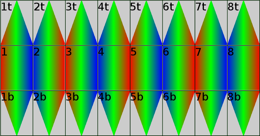
Fig. 7. pattern brightness for station 2 view 0 (top channels)
Fig. 8. pattern brightness for station 2 view 0 (top), specular component
Fig. 9. pattern brightness for station 2 view 1 (bottom channels)
Fig. 10. pattern brightness for station 2 view 1 (bottom channels), specular
Acquiring thousands of images made by different channels of the camera and capturing the same target, it is possible to perform simultaneous relative photometric calibration of the pattern and the sensors, provided that each element of the pattern preserves the same brightness for each image where it is captured. This may be true when the target is observed from the same point, but when we calibrate Eyesis4π camera with 2 sensors attached far from the other ones, and these sensors travel significantly when capturing the target, this assumption does not hold. The same pattern element has different brightness depending on the lens position when the image is acquired. This is because even matte pattern material is not perfectly diffusive, there is some specular (reflective) component.
In the earlier setup we used photographic lamps with large umbrellas, but these umbrellas were still small when placed at a distance that they were out of the camera view. Specular component was still visible when the diffusive part was subtracted. When designing the new calibration target we decided to use bright linear fluorescent lamps along the floor and the ceiling and keep them spatially compact without any diffusers or umbrellas, we only used mirrors behind the lamps to effectively double the output. Such light source was expected to produce specular reflections on the target, but these reflections occupy just a small portion of the target surface, the rest of it is close to be pure diffusive. That allowed us to locate positions of the specular reflections for each camera station/viewpoint by subtracting the average (between all stations/viewpoints) pattern brightness from each individual station/view of the pattern and then masking out this areas of the pattern during flat-field calculations.
Images on Fig. 7-10 were made for camera station 2 – 3.3m from the target and 1.55m to the right of the target center, that caused lamp reflections to be shifted to the left. View 0 (Fig. 7-8) correspond to the camera head, which is the center of rotations. View 1 (Fig. 9-10) is captured by the camera 2 bottom sensors mounted 820 mm below the camera head, so they were moving significantly between the images – that caused visible curvature on the top lamps reflection.
Virtual tour of Elphel calibration facilityYou may walk through our calibration facility using our WebGL viewer/editor. The images were captured with newly calibrated Eyesis4π camera, there is no 3-d parallax correction – these are just raw panoramas stitched for infinity and most close objects are out of depth-of-field of the lenses. Hope you’ll still enjoy this snapshot of the new facility were we plan to develop and precisely calibrate many new cameras.
Sensor+Lens Tool
There’s a number of online lens calculators already and this one is not conceptually different – the focus is on the current sensor we use and the main feature is visualization done in HTML canvas using jCanvas.
It might help to figure out what lens is needed for a particular application where certain parameters can be important, e.g.:
It might help to figure out what lens is needed for a particular application where certain parameters can be important, e.g.:
- Field of view for a lens of the given format
- Depth of field at a fixed distance and f-stop
- Aperture size (f-stop) at which the resolution starts to degrade due to diffraction limiting
- Different sensor formats (also compared to the “full frame” format)
- Circle of confusion formulae (affects hyperfocal distance and depth of field):
- 1px – for machine vision applications
- d/1730 & d/1000 – “Zeiss formula” for photography
- Distance to in-focus plane
- Lens focal length
- Field of view
- Diffraction limit for aperture size (calculated for red light of 690nm, Airy disk size equals to 1px)
- Depth of field
Links
Heptaclops camera and the 393
“Temporary diversion” that lasted for three years
NC393 camera will have significantly higher performance than the 353 and it will inherit the openness and flexibility from its predecessors. Elphel does not take orders on the custom design, but rather we try to do our best in making sure our users can do the customization themselves. The same policy would remain the same for the NC393 too – we will offer some camera options and add-ons, and in most cases it will be up to the camera users to build the camera of their dream.
Last years we were working on the multi-sensor cameras and optical parts of the cameras. It all started as a temporary diversion from the development of the model 373 cameras that we planned to use instead of our current model 353 cameras based on the discontinued Axis CPU. The problem with the 373 design was that while the prototype was assembled and successfully tested (together with two new add-on boards) I did not like the bandwidth between the FPGA and the CPU – even as I used as many connection channels between them as possible. So while the Texas Instruments DaVinci processor was a significant upgrade to the camera CPU power, the camera design did not seem to me as being able to stay current for the next 3-5 years and being able to accommodate new emerging (not yet available) sensors with increased resolution and frame rate. This is why we decided to put that design on hold being ready to start the production if our the number of our stored Axis CPU would fall dangerously low. Meanwhile wait for the better CPU/FPGA integration options to appear and focus on the development of the other parts of the system that are really important.
Now that wait for the processor is nearly over and it seems to be just in time – we still have enough stock to be able to provide NC353 cameras until the replacement will be ready. I’ll get to this later in the post, and first tell where did we get during these 3 years.
Up until 2009 we did not really bother with the optics of the cameras we made – cameras have a standard CS-mount that can accommodate C- and CS-mount lenses, available from many suppliers. We provided the electronics and software, but it was up to our users to deal with the rest. Yes, we did offer cameras with color and monochrome sensors, with or without IR cutoff filters, stocked some basic varifocal lenses – but that was virtually all. When we started to develop panoramic cameras ourselves we quickly recognized that the lenses we need just do not exist. The C/CS-mount format lenses are too big to make a compact layout of the camera (it not only becomes big itself, but large distance between the lenses cause large parallax that makes panorama stitching more difficult). The smaller M12 mount lenses (also called “S-mount”, and “board lens”) are mostly designed for the small security cameras and being cost-sensitive are not usually designed for the top performance.
We also realized that putting together multiple individual cameras to cover a panorama is not enough. All camera lenses have best resolution in the center, while closer to the corners it degrades. In many, especially small lenses the corners are substantially darker due to vignetting. And while we got used to it making photographs – in many cases it was even be considered as a useful feature to focus on the object in the center and blur and fade out the periphery, in stitched panoramas it is a disaster, as the individual lenses peripheral areas will be mapped to the middle areas of the composite panorama image.
Not being the lens manufacturers ourselves we went the path of correcting the lens aberrations by software post-processing ( “Zoom in. Now… enhance.” and later posts) – that allowed us to effectively double number of lens “megapixels”. Later we used the same pattern we developed for aberration correction to precisely correct the lens distortions. This process of camera calibration for the spherical view camera is described in my previous blogs (such as Building and Calibrating Eyesis4π) – we started to do so for the precise panorama stitching but later worked on making it suitable for the stereo photogrammetry and 3d reconstruction.
So now we have what we believe is the highest performance camera of a kind – the one that we demonstrated at SIGGRAPH-2012. We also have now precise thermally-compensated sensor front end that can be used in other applications – in an individual camera or in multi-camera setups.
One such application is
Shallow depth of field and cinema camerasFor many years now Elphel was cooperating with a group of enthusiasts who tried to adapt our cameras to use for cinema applications – and that fits very well into our vision: take our cameras and use them as clay to form something you (not us) envision. But eventually they got tired of waiting for our next model 373 camera (that they needed to support higher frame rate and larger image sensor) so they decided to develop a new camera themselves.
One of the main camera features they (and others who are interested in the cinematographic applications) needed was the physically large sensor. Such sensors allow capturing images with “shallow” depth of field (DoF) and can be used to shoot video where some objects are in focus, while others (farther or closer) need to be blurred. With the single lens systems the scale of distances where you can use DoF depends on the physical size of the sensor and with the small sensor as we use (and those used in camera-phones) are approximately 5 times (linearly) smaller than the 35-mm film frame. So what you can achieve with 35mm camera in 5-10 meter range is only possible in the 1-2 meter range with the small 1/2.5″ (~7mm diagonal) sensor – so instead of the human actors you’ll have to make animation with dolls. There are even special optical adapters that use 35mm format lens to focus image on the diffusing screen (made of wax or even fast rotating disk to make diffusing grains smaller) and then transfer the image on that screen to the small format sensor of the inexpensive camcorder. But that system still had limited resolution and was loosing a lot of light, dramatically reducing the camera sensitivity.
Three-camera setup for controlled depth of field capturing
The DoF first came as the feature inherent to the physical camera, the process of capturing the three-dimensional world on a two-dimensional media (film or image sensor). But in the artist’s hands it became a tool to focus viewer attention on the intended objects and also to show the 3-d nature of the actual world. With the modern computer animation there are no physical cameras with the lenses involved, but the depth of field is still present (like in this Sintel gallery). That means that the “shallow” DoF can be synthesized when the 3d information about the scene is present, and such information can be captured by other means – not only by the large format sensor and then the result image is rendered with synthetic depth of field. In some cases even a stereo-camera setup (a pair of synchronized cameras) can be used. Such setup is generally sufficient, if the in-focus objects are in foreground and there is nothing closer to the camera that occludes the target. But if such system is used to capture say image of a human behind the tree branches, then a single horizontal branch can close view of the human eye to both camera lenses. So regardless of how you blur the foreground objects (tree branches in this case) you will not be able to reconstruct the sharp image of the human face – there is no information about the color of the eye completely missing on both camera images. Using more cameras in the setup helps to provide more information about the objects – in our last case the third camera shifted vertically from the first two will have the information about the eye that was missing on the images from the first two cameras.
Building the 3-d model of the scene from the multiple images is not an easy task. The precision of the depth measurements is much lower than measuring distances in the direction orthogonal to the line of view. And often the portions of the scene have no fine details and so there is nothing to match to find out the distance to that object. On the other hand, when the 3-d reconstruction is needed just for synthesizing DoF, the precision of the distance needed to simulate the DoF of a real lens is the same as you can get from the lenses separated by the large lens diameter. The areas that do not have details, where it is impossible to measure distance – that areas would look the same on the final image, even if you blur them with the wrong sigma (or not blur at all).
HTML5 demoA section of the screenshot - click on the image to open the actual HTML5 demo page
We do not yet have a seven-camera setup or “heptaclops”, we used a smaller “triclops” configuration. When we had built and calibrated the new camera (using the target pattern data measured earlier with Eyesis) we looked at the way to demonstrate it. First the images were processed with the known calibration and each of the raw images was mapped to the common projection plane – each pixel with ~0.15 pix accuracy – this process compensates for the lenses distortions and mis-alignment of the individual sub-cameras. These images can be used as the input data for the 3-d reconstruction. We do not have finished 3-d processing software yet, Oleg Dzhimiev made a small HTML5 application that illustrates the information from the camera triplet.
This web application overlaps the triplet of the corrected images acquired simultaneously by the 3 sub-cameras and applies the transparencies to the two of them so the the visible superposition has equal weight of each image of the set. Then each image is shifted by the value of the disparity that matches the distance from the camera to the image plane – the amount of disparity is controlled by a slider or by rotating the mouse scroll wheel. The objects in or near the selected image plane from all three images coincide, while the objects closer or farther from the camera are shifted from each other. When the shift is small, it looks like a blur, but farther images look as they actually are – as individual ones. While these separate image spoil illusion of the out-of-focus blurring (but still looking more realistic than dual images in old rangefinder cameras), they illustrate the raw data. Using more parallel cameras would improve illusion of focusing on such fast demo and provide more data for the actual reconstruction, reduce ambiguity when finding the disparity (and so the distance) at each pixel. Additionally, combining the data from multiple individual sensors would increase signal-to-noise ratio of the result image and so the dynamic range even if used with the same exposure/gain settings. And it is possible to program some channels with different exposure and run the whole system in the HDR mode.
The same applcation can be useful with the 3-d processing too. Instead of the 3 images that are just aberration and distortion corrected originals acquired from the different sensors, we can generate multiple close views and feed them to the same program – just shifting multiple images (or videos) is much less computationally demanding as correct 3-d rendering of the scene with the selected image plane and DoF, so such application can be used as a preview for the artist to dynamically adjust those parameters (distance and DoF) before running the final rendering (when it is possible to add desired bokeh too).
Back to the Model NC373 camera status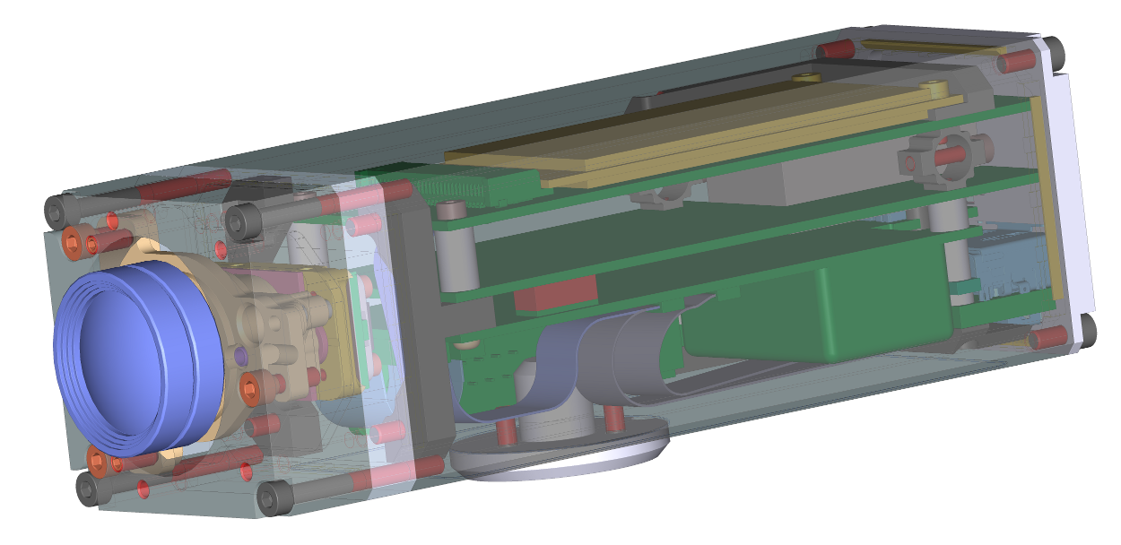
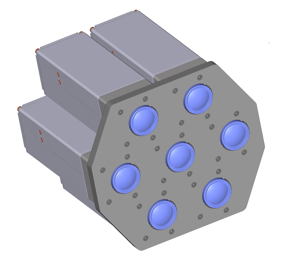
Model NC393 CAD rendering with M12 (S-mount) lens and thermally compensated sensor front end
We decided to drop the idea of building the already designed and prototyped model NC373 camera. While the next camera will share some parts with the 373, the changes are too big to call it just a revision “C” of the 10373 system board, so it will be model NC393. The camera system board will have Xilinx Zynq that combines FPGA and a dual-core ARM processor on a same chip, so my main concern of the FPGA-CPU bandwidth is not applicable here.
When information about the new Xilinx device was announced, I thought it is a good candidate for the next camera design. In spring of the last year we had a Xilinx seminar in Salt Lake City, where I was told that these new devices will be supported by the zero-cost development software.
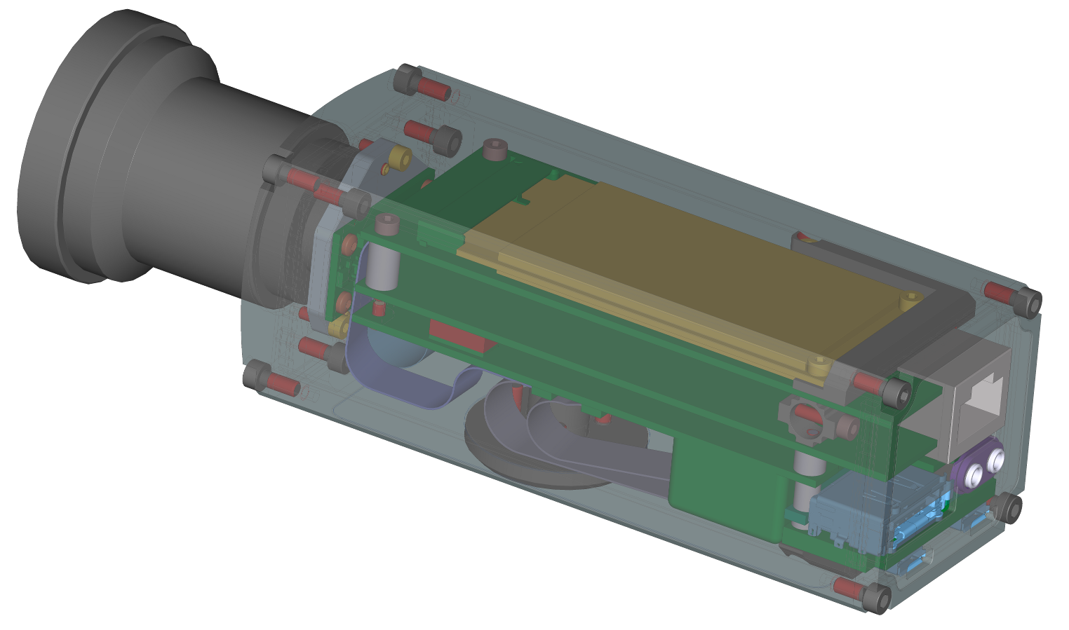
Model NC393 CAD rendering with a C/CS-mount lens
That feature is very important for us, because while the cost of the tools is not high for the manufacturer, it is higher than the cost of a camera. We strive to make our products highly customizable by the users, each camera contains the source code needed to compile the executables (including the FPGA code). Making our customers to pay high price to be able to modify even a single line of the FPGA code is not acceptable to us, so we use only those FPGA devices in our designs that are supported by the software that our users can download at zero cost. Of course ideally we would love to use free (FLOSS) development tools (like we use for the FPGA functional simulation), not just the zero cost ones, but in the real world it is not possible yet, so we develop and share our free (licensed under GNU GPLv3) code with the non-free closed-source tools.
The news that came from the Xilinx reps later last year were really disappointing – none of the Zynq devices (even the smallest one) will be supported by the zero-price software tools. And only this year it finally became official that 3 of the 4 devices is going to be supported and so we can use them. Xilinx did have some production delays, the availability schedule slipped to later dates, but I’m crossing my fingers that the needed part/package combination will actually be in production by the end of the Q1 2013.
Model NC393 CAD rendering with three M12 lenses and thermally compensated sensor front ends
While the NC393 design is far from being finished, some features are already settled and are likely to remain unchanged in the final product.
- The camera will be compatible with both parallel output sensors (such as the Aptina MT9P001/MP9P031/MP9P006 that we use currently) and the multi-lane serial sensors (such as having MIPI). The connectors will not change and the sensors used with NC353 will fit directly to the NC393 camera
- The camera system board is being designed for the multi-sensor operation. It will accommodate three sensors without the need to use multiplexer boards (like 10359 needed for NC353). Multiplexer boards will likely still be used in some cases, but the system board itself will have 3 identical sensor board connectors
- Physical dimensions of the camera and the mounting holes location on the system board will remain the same as on the previous camera models
- Camera will have a single GigE port as a main communication channel
- One serial console port with internal USB converter, so a microUSB cable will be sufficient to use system console for the software development.
- Firmware installation and update will be done by booting from the microSD accessible without opening of the camera. It will be possible to use the same card slot during normal operation for data storage.
- 512MB NAND flash as a main storage for firmware, boot source for camera normal operation.
- 1GB of the system memory made of the two 256×16 DDR3 chips.
- 512MB of dedicated video memory (not shared with the CPU) – one 256×16 DDR3 chip, same the one used for the system memory.
- USB2 (host): One external micro-USB and 2 internal flex cable connectors with USB, additional 3.3VDC power, I2C and FPGA general purpose I/O compatible withe the add-on boards for the NC353
- 30-pin board-to-board connector with 12 differential /24 single-ended FPGA I/O for add-on boards.
- a pair of 2.5mm audio connectors on the back panel for camera synchronization – from external trigger and/or from other cameras
- 2-port SATA controller based on the free (GNU/GPL) implementation. Camera will have eSATA/USB external connector (so capable of running external SATA device without additional power supply) and internal mSATA SSD that fits inside the camera.
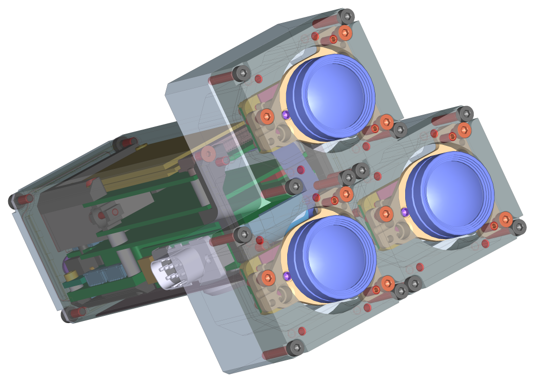
Model NC393 CAD rendering with three M12 lenses for capturing panorama images
NC393 camera will have significantly higher performance than the 353 and it will inherit the openness and flexibility from its predecessors. Elphel does not take orders on the custom design, but rather we try to do our best in making sure our users can do the customization themselves. The same policy would remain the same for the NC393 too – we will offer some camera options and add-ons, and in most cases it will be up to the camera users to build the camera of their dream.
Elphel will use the new system board in the Eyesis cameras. It will allow us to make the overall design more compact by reducing number of boards inside, increase the network bandwidth as well as the SSD bandwidth, increase the frame rate. We also plan to increase the camera resolution by switching to the same format but smaller pixel sensor while reusing the same optical-mechanical design – that would be definitely too much for the current system that is limited to the currently used sensors.
And of course we will continue to build “small” cameras based on the new design – with universal C/CS-mount and with M12 one, including precisely calibrated fixed-lens systems. And as the camera is designed for the multi-sensor operations, we will offer several typical configurations for robotic (parallel sensors for stereo-vision) and panoramic applications, as shown on the images above.
All the camera hardware documentation (circuit diagrams, parts lists, PCB layout and mechanical CAD files) will be released under CERN OHL license when the design will be finished and we will start the actual production of the cameras (add-on documentation will be released when it will become available) . All the firmware and FPGA code will be traditionally released under GNU GPL and maintained at Sourceforge repositories.
Building and Calibrating Eyesis4π
This is a long overdue post describing our work on the Eyesis4π camera, an attempt to catch up with the developments of the last half of a year. The design of the camera started a year before that and I described the planned changes from the previous model in Eyesis4πi post. Oleg wrote about the assembly progress and since that post we did not post any updates.
Working on the first camera of this series we had to solve several technical problems – and that push us back behind our schedule. First problem was with the use of the UV-curing adhesive to fix the sensor relative to the lens. In the first Eyesis we incorporated some elements of the sensor adjustment into each SFE (sensor front end), in the current system we decided to follow a more traditional approach and adjust the sensor on a specialized device and then fix the position with the adhesive – that allowed us to make the SFE more compact and we hoped to simplify it too. In the new design I tried to reduce the thickness on the UV-curable adhesive and make the system self-compensating for the glue shrinkage during curing and thermal expansion of it when the camera is used. The solution used 3 pins in 3 holes with the glue between the pins and the walls of the holes, so expansion/contraction of the adhesive would not lead so significant movement of the pins. Unfortunately the illumination of the glue with the UV radiation proved to be insufficient (some shadow areas remained) and the UV LED were on the same side of the glue where it contacted the air, so the most illuminated areas suffered from the “oxygen inhibition”. We tried several small modifications but still could not achieve reliable and strong bonding we needed. So we decided to use just low-shrinkage epoxy instead of the UV glue the first camera and leave more radical redesign for later time. With epoxy we could make only 2 SFE in 24 hours, because the curing took much longer than the UV glue and we could not use fast-setting epoxy as the adjustment took some time. That method was slow but it worked. Worked until we decided to measure the temperature dependence of the focusing and realized that just maintaining the SFE “in focus” over the intended temperature range is not sufficient for our application where we compensate for the lens aberrations with post-processing. The measured temperature coefficient was about 0.2μm/°C – that corresponds to 10 mm of the expanding aluminum – material used in most of the SFE.
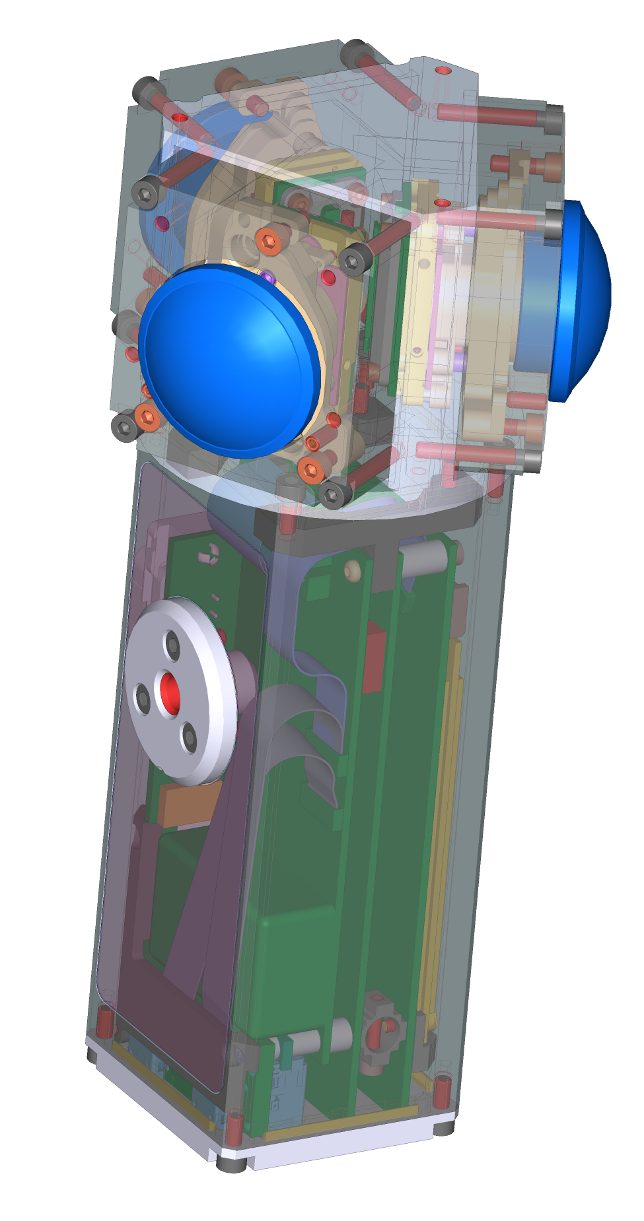
Thermally compensated SFE design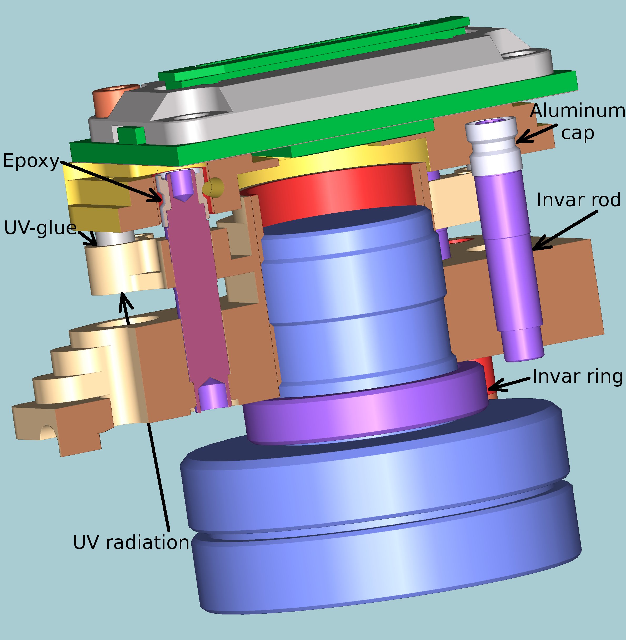
Section of the SFE used in Eyesis4π
We could not think of any quick fix to that problem so we decided to go through the complete redesign of the sensor front ends used in Eyesis4π cameras, add thermal compensation and improve bonding process. Some elements of the SFE are made of invar – nearly zero expansion material for the thermal compensation, the bonding is spit into two separate stages – fast UV bonding and final using low-shrink epoxy. Additionally we modified the 10338D sensor front end PCB (the new version has revision “E”) to include the temperature sensor. Luckily for us we just had to replace a single chip – instead of the serial EEPROM the new board uses a combination of the EEPROM and a temperature sensor in the same size package and pinout (such chips are used in computer memory modules to store module parameters and monitor temperature). The new board simplifies temperature dependence measurements of each SFE during manufacturing, it also makes possible to do perform additional thermal correction of the acquired images – the SFE temperature during acquisition is embedded in the Exif header of each of them.
The 0353-07-25 SFE has two major parts – the base with the attached lens and the movable (during adjustment) plate to which the sensor PCB is attached. These two parts are connected with the 3 invar rods, each being press-in (and then flared) in the base. Only the very bottom part of the rod is press-fit, most of it is loose so the thermal expansion of the aluminum base is isolated from the rod. The base has 3 arms that are partially cut through to allow some bending, these arms support the invar rods laterally while allowing the axial movement caused by the thermal expansion. The top of each invar has aluminum cap pressed on and flared, these caps fit (with the sufficient clearance to guarantee co-contact during adjustment process) inside the holes in the sensor plate and are later bonded with the epoxy compound. Each of the 3 arms that provide lateral support of the invar rods additionally have 3 through holes that are temporarily plugged at the bottoms with the transparent adhesive tape to hold UV-curable adhesive. The sensor plate has 3 thin-wall stainless steel tubes pressed in it, these tubes are immersed in the adhesive and bonded to the base arms when irradiated with UV from the bottom during curing. The SFE is mounted in the adjustment machine with the lens pointed down, the mirror mounted at 45 degree reflects the target pattern located on the vertical wall. The same mirror reflects the UV radiation during curing process after the adjustment is finished. The 2.8mm invar spacer ring (for expansion it is in-series with the rods) is designed to slightly over-compensate the thermal expansion of the aluminum parts, so it can be made of different material (or a combination of 2 washers made of different materials) to fine-tune the overall expansion. This design allowed to reduce the thermal variance of the distance between the sensor and the focal plane of the lens by nearly an order of magnitude – the measured value falls in ±0.03 μm/°C range.
SFE compensated for the purpose of the aberration correction that maintains the same position of the lens focal plane relative to the sensor surface still has some magnification variations caused by the sensor expansion itself among other factors. It is not large – until we upgrade camera to the higher resolution sensors the change for 10°C is only 0.08 pixels for the diagonal corners of the image, this effect can be easily compensated when the temperature during acquisition is known.
Camera calibration machine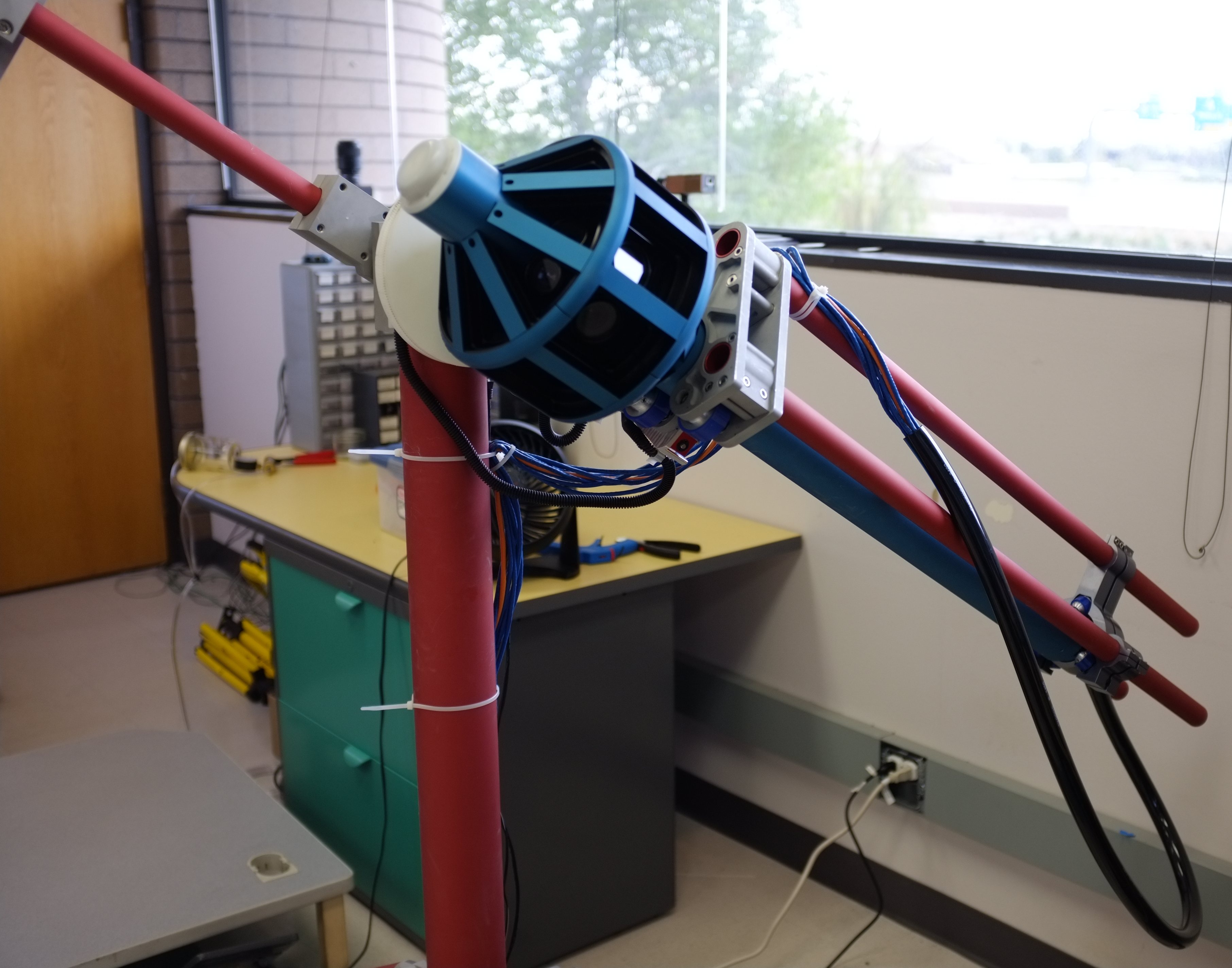
Goniometer with Eyesis4π camera
Camera calibration involves the following procedures:
- measuring the point spread function (PSF) for each area of the field of view of each sensor to be able to compensate for the aberration during post-processing of the acquired images
- measuring distortions of each lens and precise orientation and position of each lens in the camera assembly so the result images have the pixels precisely mapped to the lines in space
- measuring the vignetting of each lens including variations of color reproduction over the area of each sensor
- logging the inertial measurement unit (IMU) data
All the optical measurements (first three) are made with the same target pattern described in the earlier post. When performing the distortion measurements the camera can be located rather close to the pattern, but for the aberration measurement and correction it should be within the depth-of-field range from infinity – distance at which the camera will operate. In our case it is 6 meters. With the individual sub-camera FOV of 45°x60° the target pattern would have to be 5m (horizontal) by 7m (vertical) to fill the sensor completely. As it is not easy to make and use such large target we developed software to combine PSF data from multiple overlapping images of a smaller pattern – we used 3022mm by 2667mm that fits on the wall in our office.
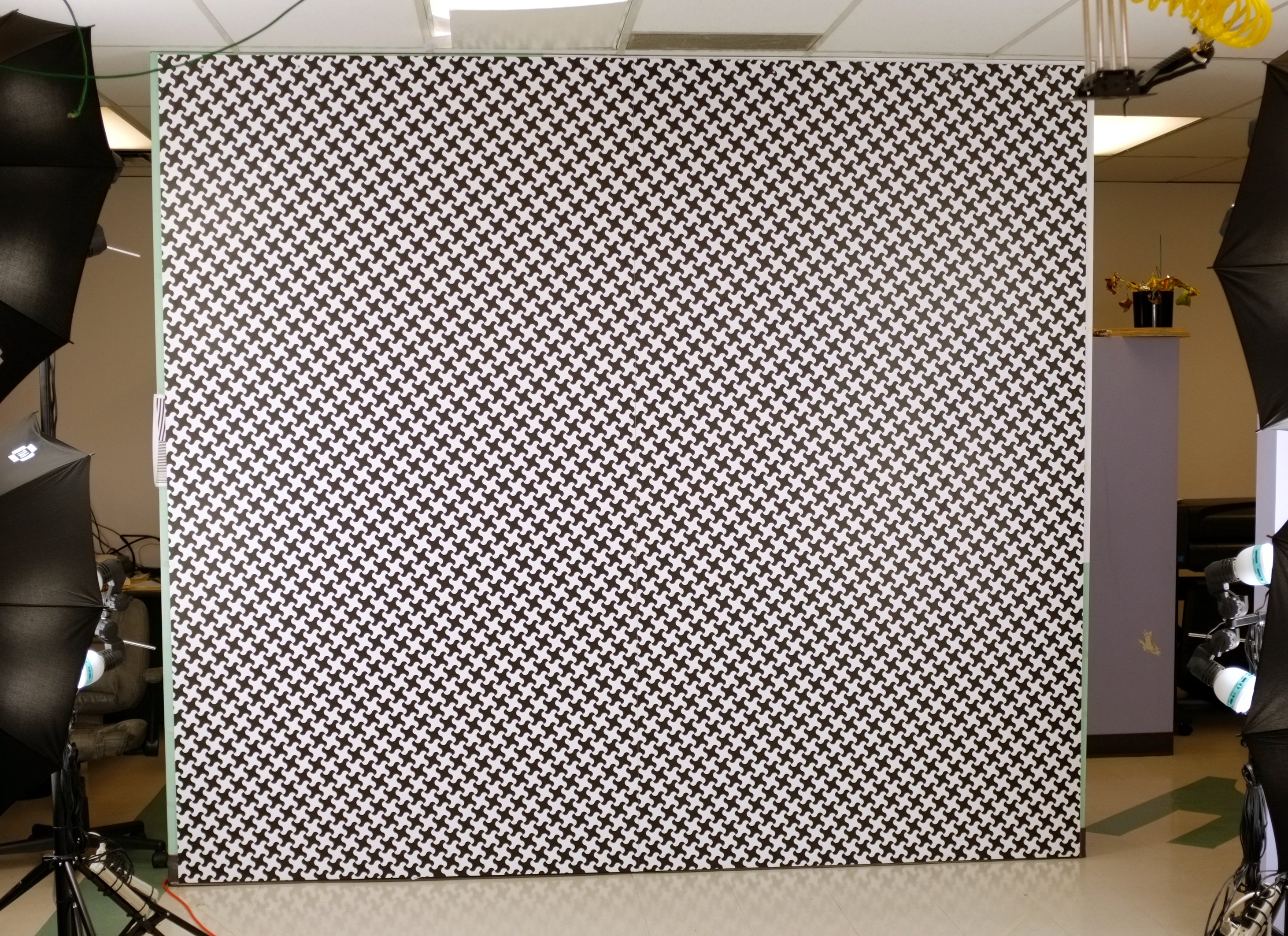
Calibration pattern
When calibrating the earlier Eyesis model that had just 9 sensors we manually rotated the camera on a photographic tripod and were making at least 12 shots for each sensor. For the Eyesis4π with full sphere FOV and with the long tube body that can not be detached during calibration (it has essential electronic boards and the two bottom sensors on it) the regular tripod would not work. So we had built a special device that allows rotation of the camera around to axes – horizontal (it goes approximately through the center of the camera optical head) and the vertical axis of the camera. As the camera is capable to view at nadir (along the tube body) the camera is rotating in the polyurethane rollers that do not block the view of the target along the tube.
When the PSF are calculated during post-processing it does not matter what part of the pattern is visible – the ideal pattern is locally distorted for the best fit with the acquired images and then used in deconvolution to calculate the aberration correction kernels, minor geometric errors in the pattern and non-flatness of the pattern surface are not critical. But the same is not true when we perform the distortion measurements and precise pixel mapping – in that case the stretching of the pattern panels, non flatness would cause significant errors. In this case the pattern is treated as a 3-d mesh of the pattern cells with arbitrary coordinates of each of the nodes, these coordinates are determined during bundle adjustment with the camera parameters. The post-processing in this case should not just fit ideal pattern to the measured images, but have an absolute match (same cell to the same cell) between the wall pattern and the acquired images.
There are several methods to achieve such matching. One is to add special marks to the pattern or just some non-periodic elements that would allow unambiguously determine what part of the whole pattern is visible. That would work for the purpose of the PSF measurement – if the pattern marks are recognized they can be included in the simulated pattern being used for de-convolution. We used a different approach – projecting spots by the 4 red diode lasers to the white pattern cells at some distance from the corners.These lasers are under software control so multiple images with different state of the lasers are recorded and used for absolute matching of the actual and acquired pattern, the final image is made with all lasers off, so pattern is not influenced by them.
The distortion calibration for individual sensors is described in an earlier post – Subpixel Registration and Distortion Measurement – it uses Levenberg-Marquardt algorithm (LMA) to simultaneously fit the whole camera orientation/position as well as individual lens/sensor parameters. The calibration machine allows acquisition of multiple sets of 26 simultaneous images, for the full calibration we record about 450 sets to have good overlap – each area of each sensor has the target visible on at least 4 images, after filtering out images that did not capture the view of the target pattern there are about 1500 images to process. It is essential that while the overlap between different sensors FOV is small (under 10%) the same target pattern is visible by multiple sensors on many image sets images, this allows to determine mutual location/orientation of the sub-cameras and finally find out the coordinates of each lens in the camera coordinate system.
Before the image data is processed farther, these images are converted to arrays of pattern grid pixel coordinates using absolute grid cell numbers if laser pointers were detected or just relative if the pointers are not available. Images without laser pointers data are still useful – they are processed when the program has enough information (from another images) to predict where the pattern nodes are expected.
The calibration measurement takes about 10 hours – the laser pointers are detected from 6 images (to increase signal-to-noise ratio) and those images are discarded, only a single images with laser pointer metadata is preserved, this processing accounts for the most of these 10 hours procedure. We perform it overnight to reduce requirements to completely block the daylight and avoid disturbance from shaking the floor. And still the processing discovers small number of images that do not fit with others (usually by under 0.3 pixels) – that is most likely caused by semi-trucks going over the speed bump right by our building. Luckily such disturbances are present on very few images and it is easier to use software to detect and remove them than to provide a complete vibration-free calibration environment.
Parameters that are determined during fitting with LMA include:
- position and orientation of the calibration machine relative to the target,
- distance and angle between the two camera rotation axes,
- locations and orientations of the individual lenses relative to the camera coordinate system
- lens (distortion) parameters for each channel – focal length, lens center coordinates, radial distortion polynomial coefficients and
- the two rotation angles of the calibration machine
All the parameters but the last ones (the two rotation angles) are assumed to be the same during the calibration process, the last ones are individual for each calibration set. Overall there are sup to 1500 of the simultaneously optimized variables using five to six millions data points of the reprojection error – differences (measured in pixels) between the pattern grid nodes on the images and the ones calculated from the actual target nodes coordinates and the camera model. When the algorithm converges to a set of parameters, we calibrate the target pattern itself. this is needed because the calibration pattern is printed on the material that can stretch and is not perfectly flat. Target calibration involves measuring and recording 3d coordinates of each cell, this is done by multiple iterations of referencing reprojection errors from multiple images to the individual pattern cells, calculating and applying those corrections and then repeating the LMA. After several iterations the root mean square (RMS) of the reprojection error reaches 0.3-0.5 pixels. At this stage the lens focal length, center and the radial distortion coefficients (fifth-degree polynomial) are frozen and the program encodes the residual differences as an array of X and Y corrections over the area of each sensor. We also repeat this procedure several times interleaving it with LMA that excludes the “frozen” lens parameters. This additionally reduces the RMS error down to 0.07-0.09 pixels.
Flat-field data for each sensor is measured to compensate for the lens vignetting and minor color variations caused by the sensor mosaic filter, it does not include individual pixel differences. Such data is measured with the same calibration pattern as aberrations and distortions. With the camera rotation steps we use the pattern is visible in each of the sensors in some 30-40 individual shots, each centered at different areas of the target. Assuming constant illumination intensity between measurements this allows to calibrate the relative illumination (and color variations) of the target cells and then use this data (averaged over all sensors) to determine each sub-camera sensitivity over the FOV.
Results of the camera calibration are stored separately for each of the 26 individual sub-cameras as multi-layer TIFF files with the text metadata that includes parameter values and description. These files are later used during raw image correction for precise pixel mapping and flat field correction. These files include:
Lens residual distortion, x-coordinate
- short text description of each parameter
- sub-camera (channel) number
- position and orientation in the camera coordinate system
- optical parameters
- Focal length
- Coordinates of the lens axis
- Radial distortion coefficients
- and the following six 2-dimensional arrays stored as image layers (1/4 resolution of the sensor):
- Residual horizontal (X) correction in pixels (shown on the illustration
- Residual vertical (Y) correction in pixels
- Image mask
- Red color channel sensitivity (divide raw picture by these values for correction)
- Green color channel sensitivity
- Blue color channel sensitivity
FOV of sub-cameras in Eyesis4π, colors show relative time of the pixel acquisition (from red to blue). Same colors designate simultaneous capture.
Image mask is used to specify which parts of the sensor provide useful data, sensors covering areas around zenith and nadir acquire only triangular segments of the full sensor rectangular pixel array as shown on the picture to the left.
This earlier article explains why using only 50% of the area of those sensors is not a waste but helps to avoid stitching problems caused by fast movement of the camera visible on some high-resolution footage from car-mounted panoramic cameras that use sensors with electronic rolling shutter similar to Eyesis.
Rolling shutter can still cause image distortions in Eyesis but such design guarantees that there will be no duplication or even worse – gaps in the areas where images from different sensors are merged together. When the imagery is used for just rendering panoramas, those residual distortions are not visible (unless the camera was shaken really violently during image capturing). If the same image sets are intended for the photogrammetric applications the rolling shutter effect has to be dealt with to keep the total error in subpixel range, comparable with that of the static camera calibration. Such correction relies on measuring the camera egomotion with the embedded inertial measurement unit and applying camera position/orientation at the moment when each pixel was acquired to the static pixel mapping.
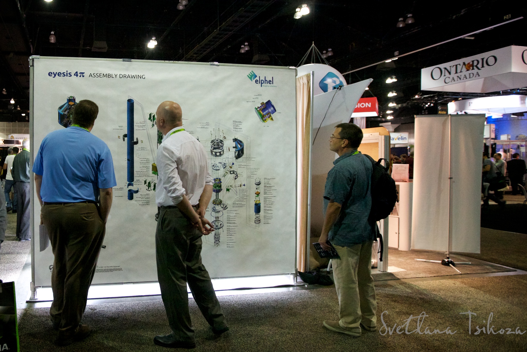
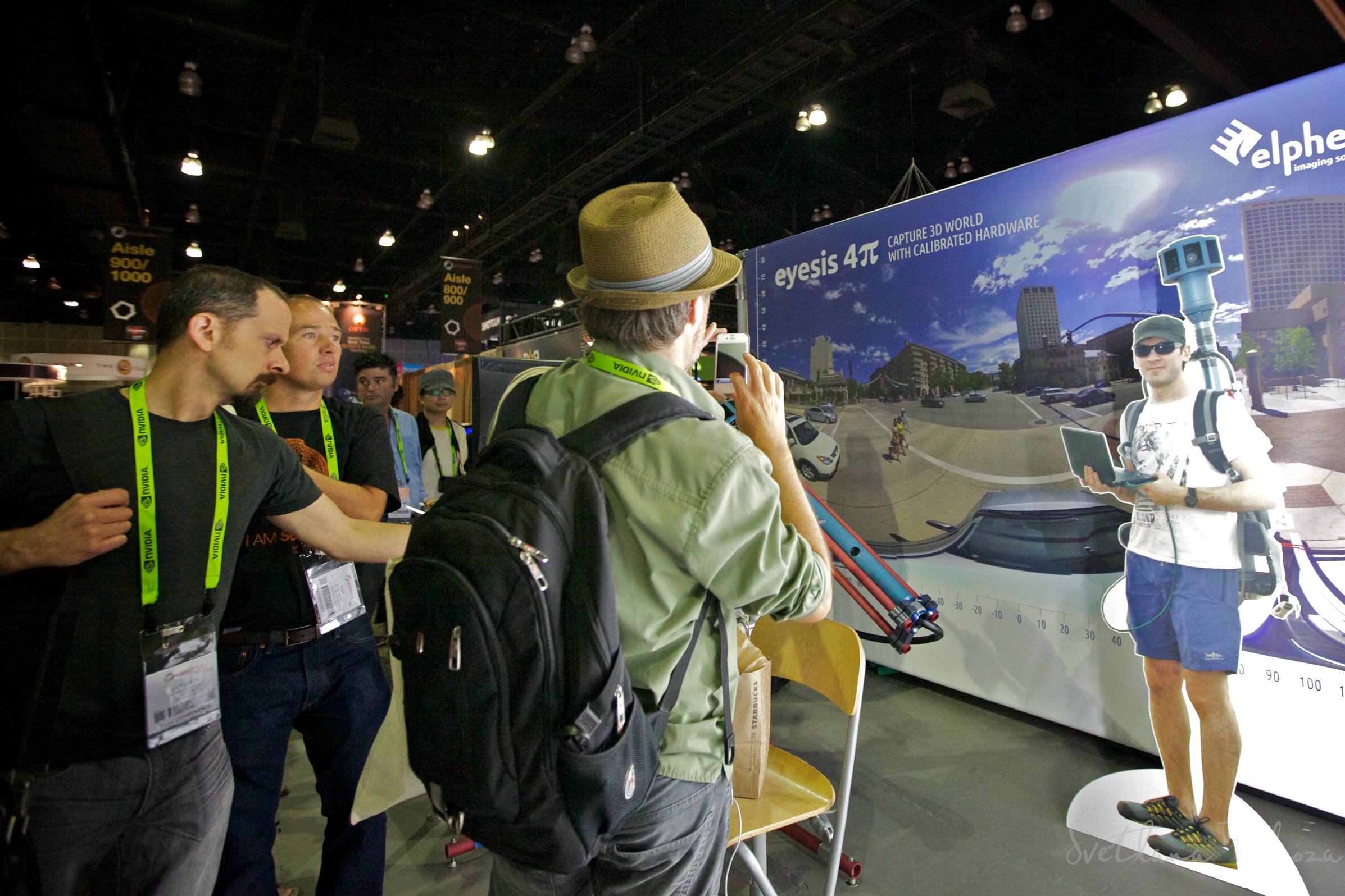
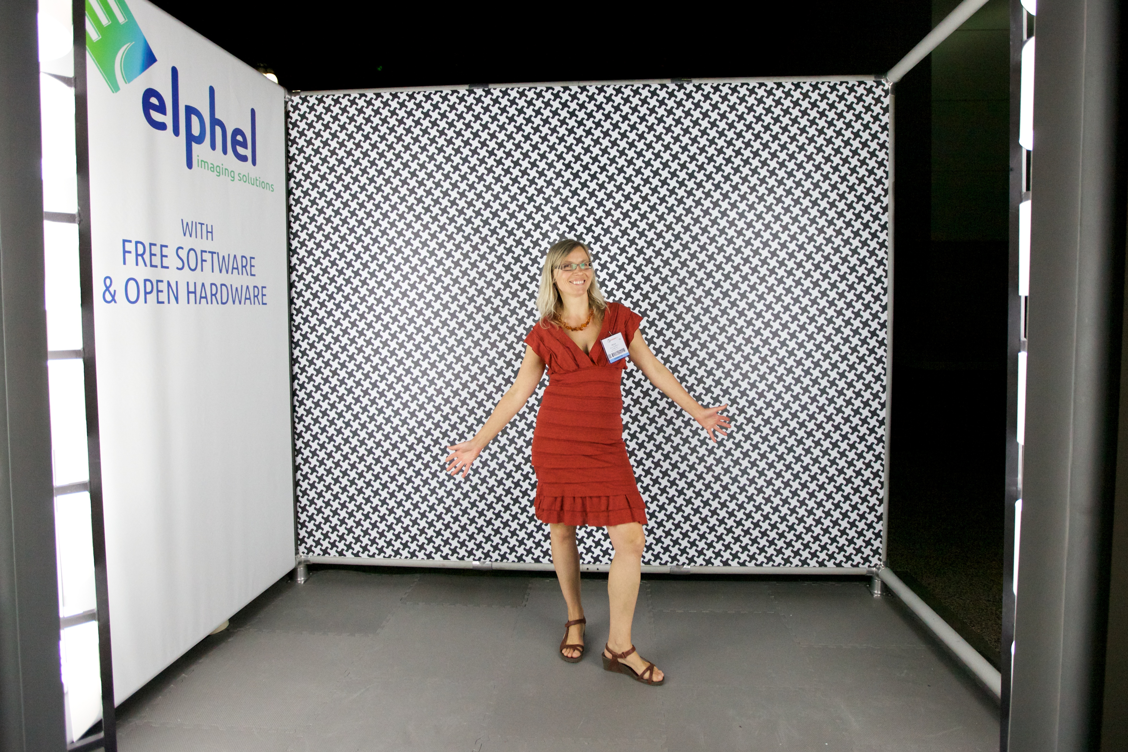
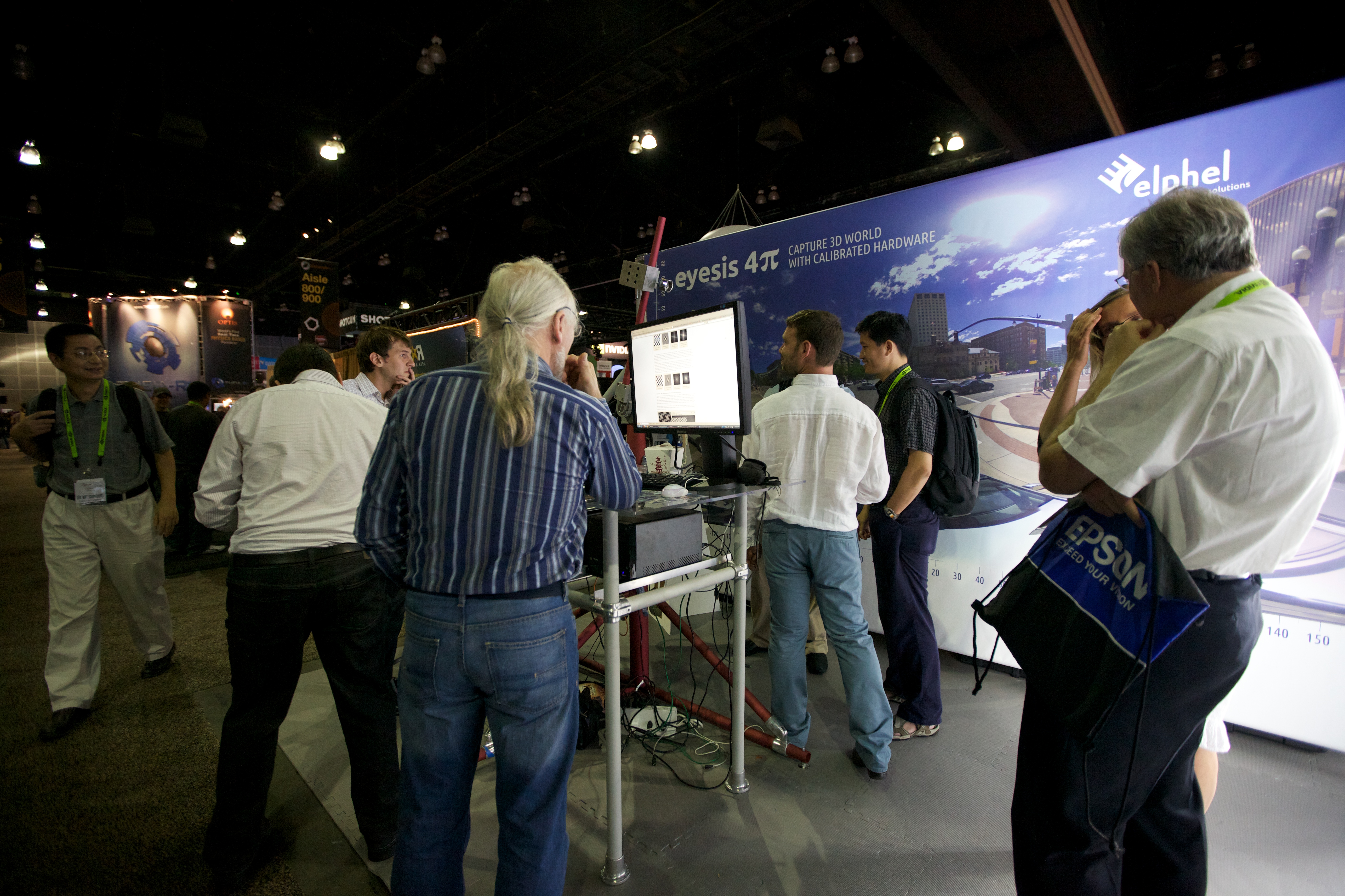
The last chance to see us at SIGGRAPH’12
Thanks to everyone who had visited us, learned about Eyesis4Pi and suggested some new applications. We hope you have enjoyed our discussions as much as we did.
We are glad to see so much interest in the Eyesis4π panoramic applications we have demonstrated and we continue to look for collaboration in 3D reconstruction based on our camera calibrated for photogrammetry.
We are glad to see so much interest in the Eyesis4π panoramic applications we have demonstrated and we continue to look for collaboration in 3D reconstruction based on our camera calibrated for photogrammetry.
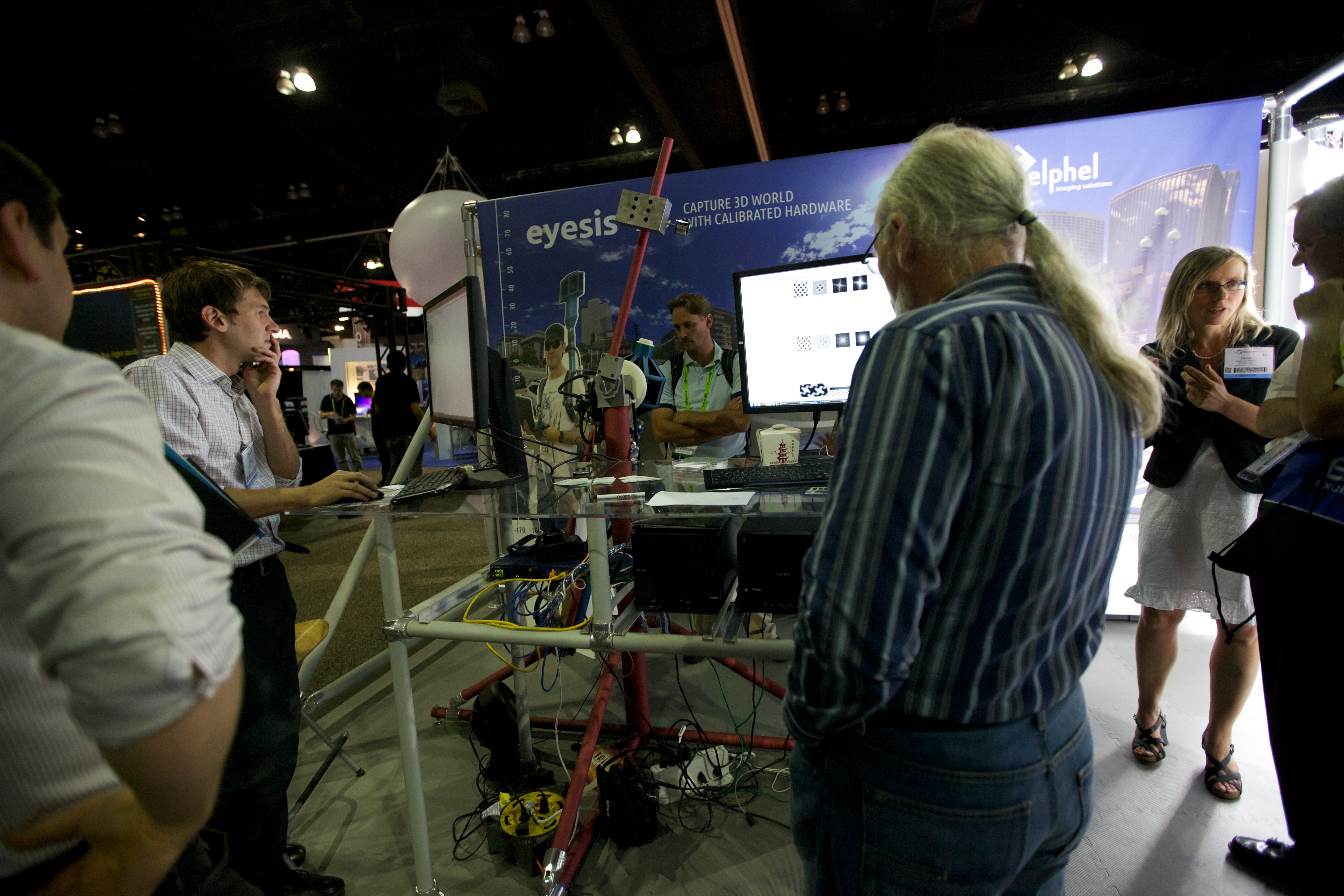
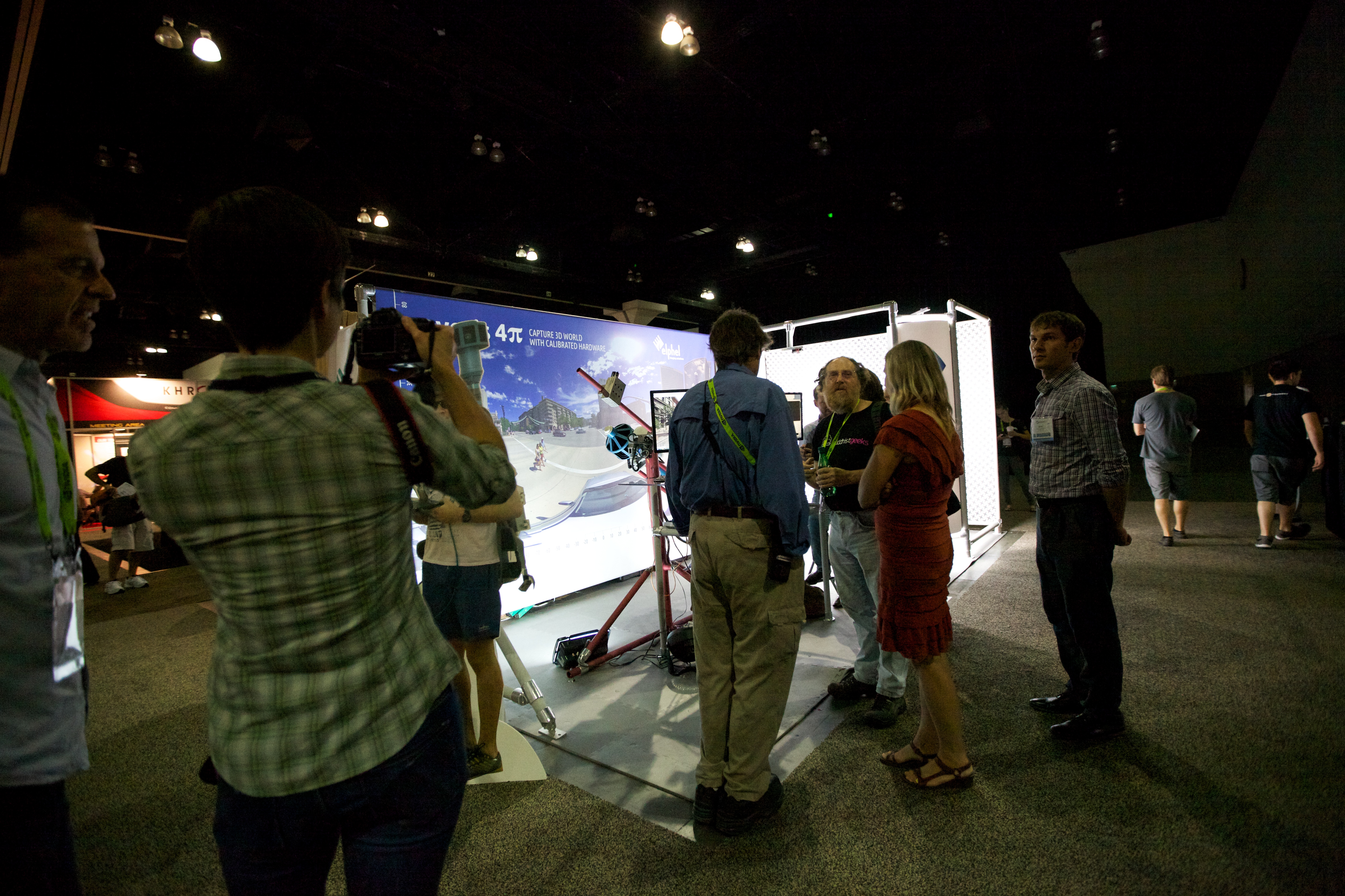
Elphel at SIGGRAPH 2012
Tuesday August 7th – Thursday August 9th
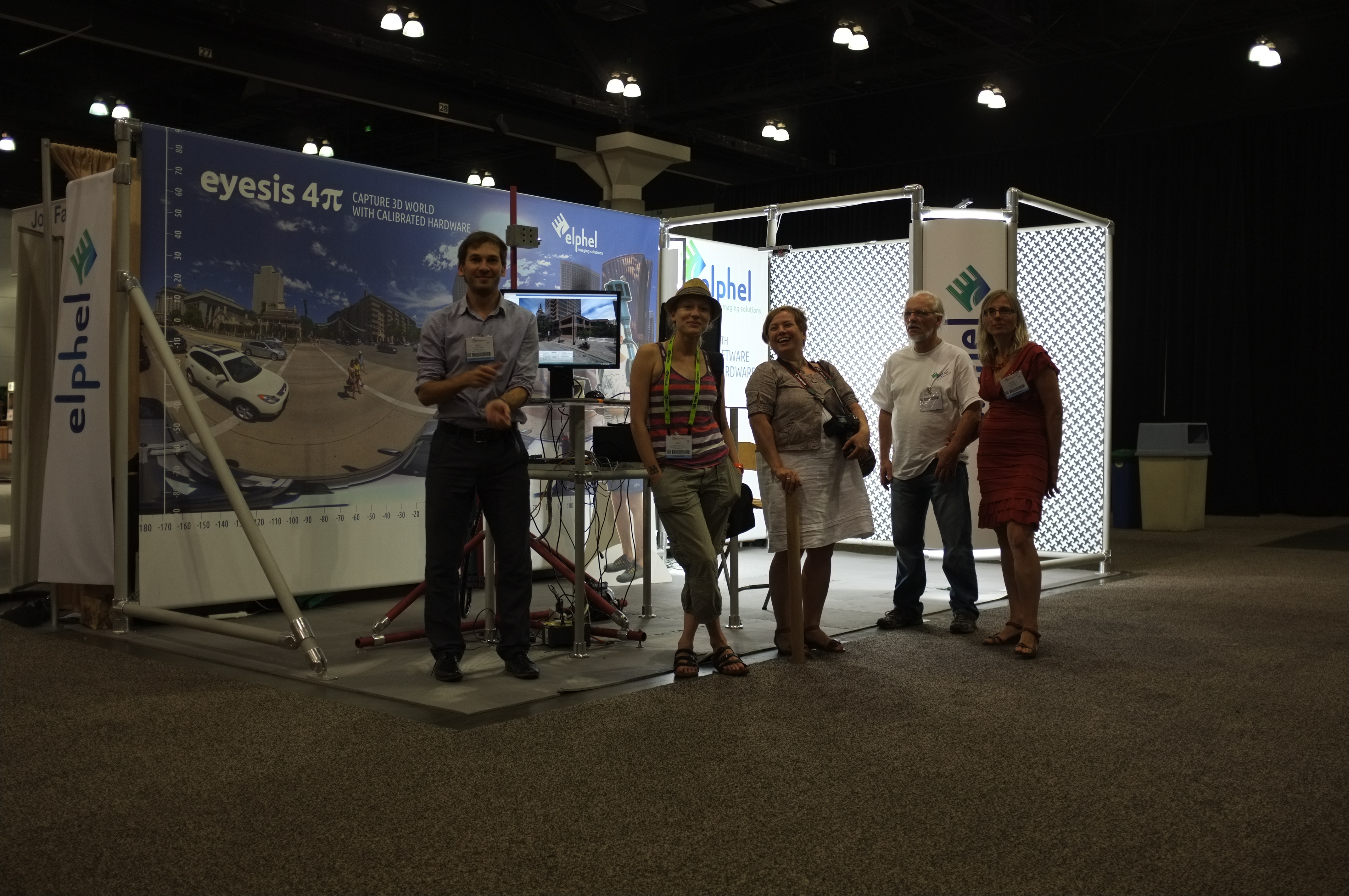
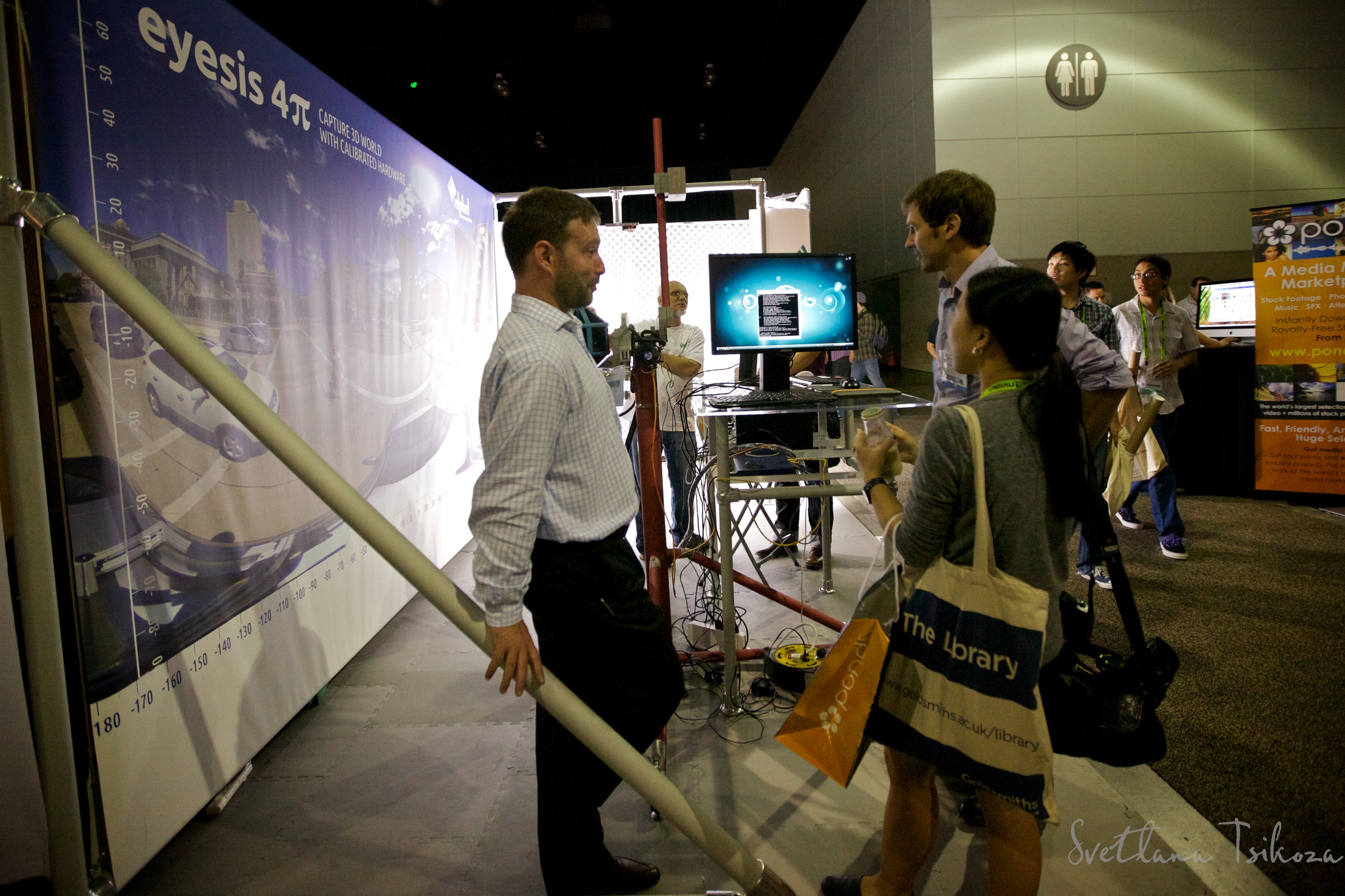
Los Angeles Convention Center, Main Hall , Booth 1058
Elphel will present Eyesis4Pi – high resolution full sphere stereophotogrammetric camera at SIGGRAPH 2012, together with it’s calibration machine. We will demonstrate full calibration process to compensate for optical aberrations, allowing to preserve full sensor resolution over the camera FOV, and distortions – for precise pixel-mapping for photogrammetry and 3D reconstruction.
All Elphel camera users are welcome, current and prospective, as well as parties interested in Eyesis4Pi. Here (booth 1058 – see plan) you can talk to the camera developers, see the calibration process and touch the actual working hardware. There is a number of passes available for exhibition only. Please contact Olga Filippova if you would like to receive one.
Run ImageJ plugins from the command line in Ubuntu
1. Get X Virtual FrameBuffer
sudo apt-get install xvfb
2. Launch ImageJ (“cd” to the ij.jar directory):
Xvfb :15 &
DISPLAY=:15 java -Xmx12288m -jar ij.jar -run "TestIJ Plugin"
Comments:
- TestIJ Plugin is the name of the compiled plugin in the ImageJ menu. No need to specify a subfolder.
- :15 is an example.
Links that helped:
HomeSide 720° – A helmet mounted panoramic camera
Seeing the impressive images of the Elphel-Eyesis 4pi camera I thought it’s time to tell you about the HomeSide 720°. Like the Eyesis its purpose is to capture panorama frames with a framerate of 5fps. The major difference is that the HomeSide 720° is mounted on a helmet. To have an acceptable weight it consists of only two instead of eight Elphel 353 delivering one forth of the resolution the 4pi does. Thus the camera is able to record 30MPix frames before stitching. Additionally it’s reconfigureable to enable HDR panorama frames.
More interesting probably is the purpose it was built for. We created the assembly for indoor virtual tours. After several drawbacks we finally have an approach which works very well. We do auto leveling, auto stabilization and path extraction by image analysis only. Furthermore we recognize crossing points where the user can decide where to go when the tour is shown in the player.
This is not so easy since we neither have GPS nor IMU data. Nevertheless its possible.
All this information goes into our new webplayer which reassembles the images to a virtual tour.
Have a look at the HomeSide 720° Virtual Tour
Click into the player and use the cursor keys to navigate. You may also click and drag to change the point of view. This tour was recorded with 10MPix i.e. one Elphel 353 with two sensors.
Important: The pi symbols shows a rendered tour, not recorded by the camera
At the moment we are improving the image quality. We are also looking for a partner to drive the development even faster to create stunning indoor virtual tours.
Introducing the River View Web Player & Other News from River Studies
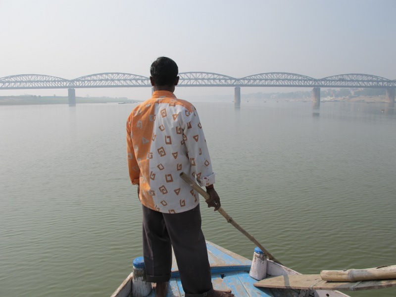
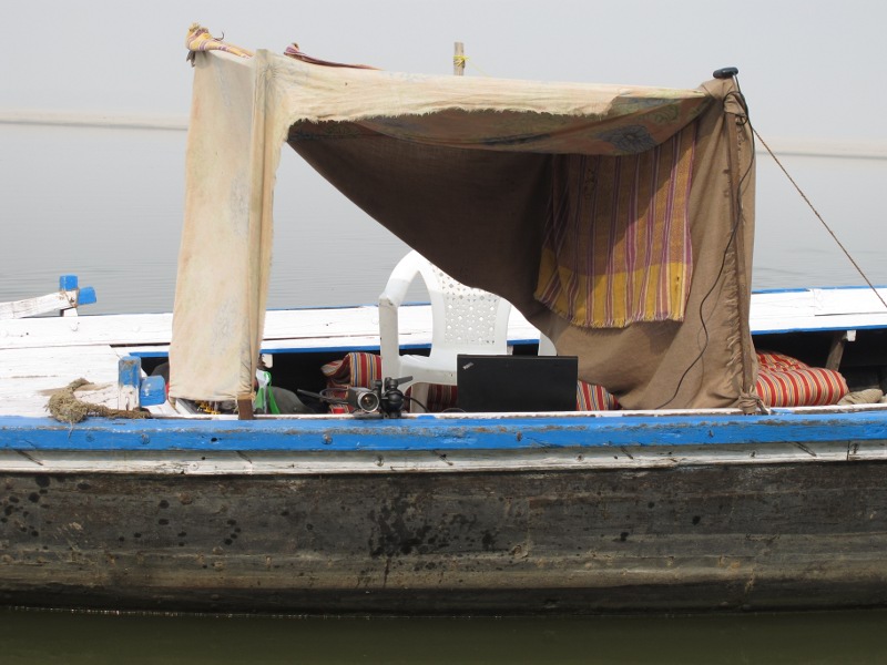
It has been a long while since my last blog entry in regards to river view panoramas. In the meantime the recording setup runs basically stable (putting aside minor problems with loose connectors) even under rough conditions (see also the gallery “Making Of” at the end of this post).
I just came back from artist-in-residency stays in Varanasi/Benares and Guwahati in India, that enabled me to have a few extensive recording sessions on various vessels like house boats, motor and rowing boats on Ganges River – for one the most sacred river to Hindus and probably most worshipped river on the planet, next to being one of the most polluted rivers of the world – and Brahmaputra River in Assam.
Many thanks go to Kriti Gallery in Varanasi and the Periferry project in Guwahati for hosting me and helping me to get onboard.
Web PlayerMeanwhile I also just finished the “River View Web Player” as a public online Beta Version. It runs on openlayers and geodjango and features the growing archive and collection of river views (up to now including views of Ganges, Brahmaputra, Danube and Nile River). There are still plenty of things to polish up, some image material to be retouched and/or uploaded, but see yourself here:
River View Web Player
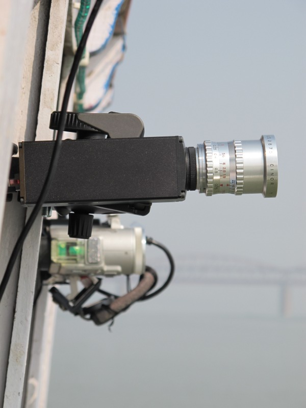
Using ElphelI am using an Elphel 353 equipped with 8 or 16mm movie lenses from the seventies to acquire this imagery. The camera delivers a Window-of-Interest video stream of 2592 x 48 pixel size with a variable frame rate between 1 and 300fps (changed on the fly according to the speed of the vessel and distance to the object of focus. That is done manually and under visual control: similar to the auto-focus mechanism, it is also a question of choice and decision and therefore not easily automatable).
The video stream is then processed and saved by custom software.
I am not using Elphel’s internal linescan/photofinish for now, since it still behaves pretty unstable and unpredictable when changing parameters like TRIGGER, VIRT_KEEP and VIRT_HEIGHT on the fly. Also, having a line per frame allows me for a more fine-graded control and preview as long as enough frames are delivered.
Elphel’s internal linescan mode, however, works quite well and stable if it runs as fast as it goes or once you have fixed a setup – as some testing on Austrian Highways prove (find more here):
Elphel 353 in Linescan mode on Austrian Highway A1 - approx. 120km/h, 2000 lps
SourcesThe source code of both, my recording software malisca and the web app and player, are open on my github repository.
Making Of / GalleryA brief guided tour to Ganges and Brahmaputra river recordings in pictures:
On Ganges
Elphel on Ganges River
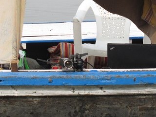
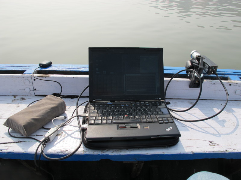
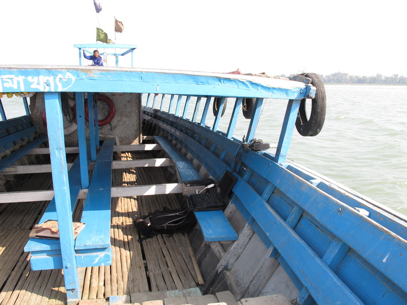
river recording setup: Thinkpad, Elphel 353, battery pack and USB-GPS-receiver
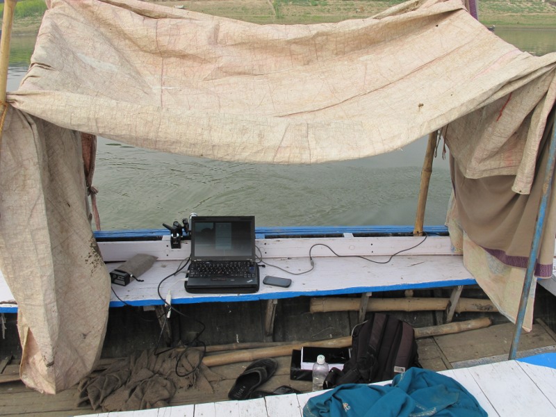
another shot of recording setup (including an improvised tent)
.. staring into the lens ..
.. obstacles (pontoon bridge) ..
lunch break on Ganges River
Elphel on Brahmaputra River
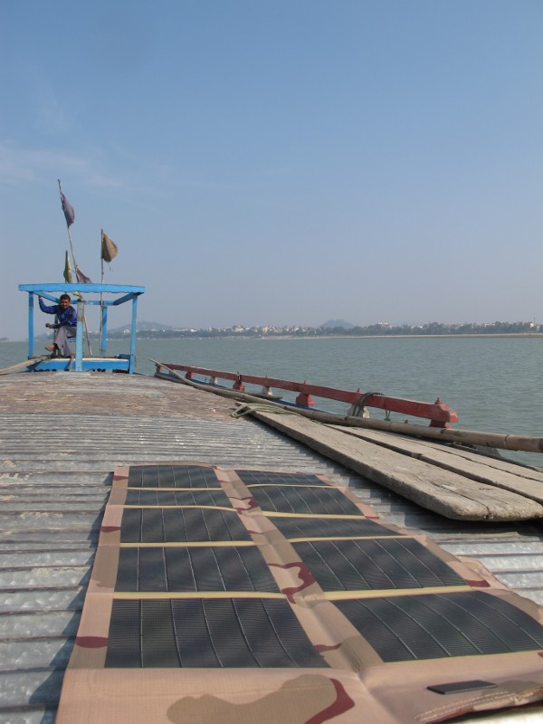
Not yet, but I would love this setup to be powered by solar energy ....